UFR 4-18 Test Case

Flow and heat transfer in a pin-fin array

Front Page

Description

Test Case Studies

Evaluation

Best Practice Advice

References

Test Case Study

Brief Description of the Study Test Case

The experiments by Ames et al. (2004, 2005, 2006, 2007) described later in this section deal with the flow of air around 8 staggered rows of 7.5 heated pins (see figure 4), spaced at P=2.5D in both stream-wise and span-wise directions (based on center to center distances). The diameter of the pins is set to 0.0254 m (1 inch) and the channel height is twice the diameter (H=2D).

The Reynolds number $Re_{D}$ is based on the pin diameter and the average gap bulk velocity. Three Reynolds numbers have been tested : $Re_{D}=3,000$, $Re_{D}=10,000$ and $Re_{D}=30,000$.

The bottom wall is heated with a constant heat-flux whereas the other walls are adiabatic. All the flow properties can be taken constant, the Prantl number is equal to 0.71. The flow is incompressible. The experimental data which have been used in the present work can be downloaded in section "Experimental results used for the CFD evaluation" below.

Figure 4: 2D Sketch of Ames et al. experiment

Test Case Experiments

General Description of the experiment

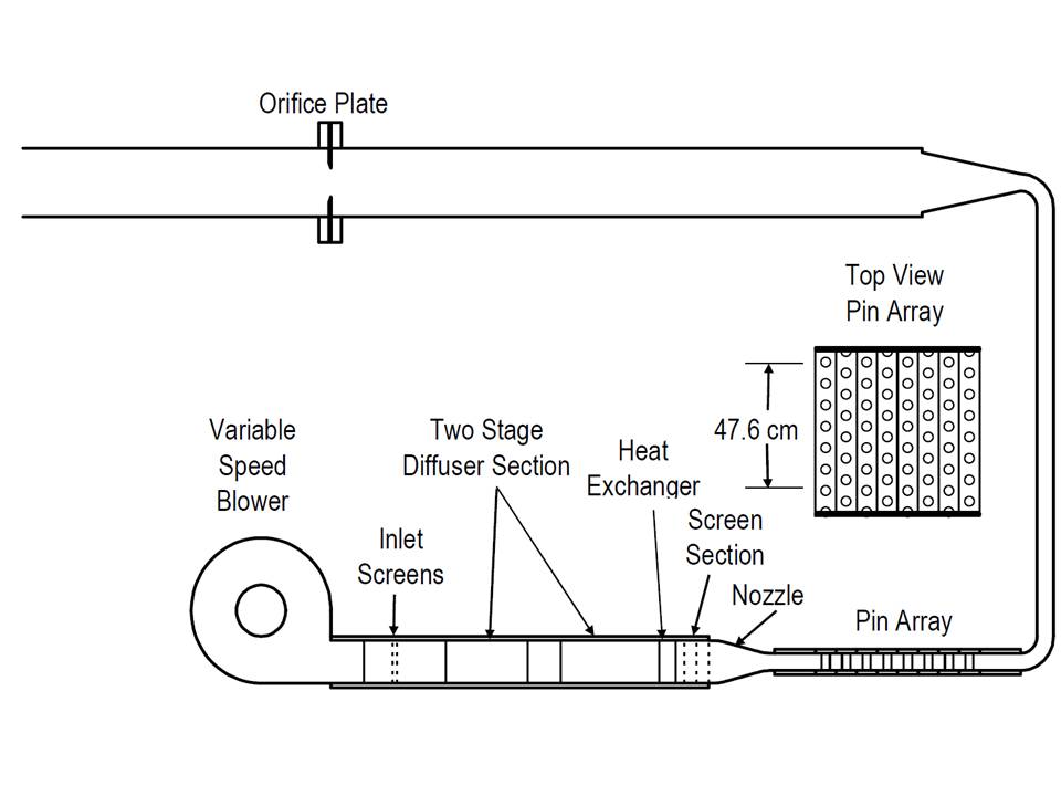
The description provided here has been given by F. Ames during the $15^{th}$ Ercoftac SIG15 Workshop. More information can be found in Ames et al. (2004, 2005, 2006, 2007). The objective of the experiments was to create a database that includes heat transfer distributions on the pin fins and endwall, pressure distributions on the pin fins and endwall, documentation of turbulence intensities and scales, and measurements of turbulence and velocity distributions across the channels. The research was conducted in a small bench top wind tunnel (see Figure 5) which included a small blower capable of producing a flow of 0.3 m³/s at a static pressure rise of 2000 Pa. The pin fin array was designed in an 8 row, 7 1/2 pin per row staggered arrangement. Both the cross passage (S/D) and stream-wise (X/D) pin spacing were equal to 2.5 while the pin height to diameter (H/D) was 2. The pin diameter was chosen to be equal to 2.54 cm. The flow conditioning system first spreads out the flow from the blower to the width of the array using a two-stage multi-vane diffuser. A heat exchanger was installed in the system downstream from the diffuser to control the tunnel temperature in order to impose a constant value. The heat exchanger discharges the flow into a screen box consisting of three nylon window screens to reduce the cross stream velocity variations in the flow. Directly downstream of the screens, the flow enters a smooth 2.5 to 1 area ratio nozzle prior to entering the test section. The pin fin array test section begins 7.75D upstream of the centerline of the first row of pins and ends 7.75D downstream of the centerline of the last row of pins. The inlet total temperature and pressure and static pressures were measured 5D upstream from the row 1 centerline and the exit static pressures were measured 5D downstream from row 8. Downstream from the test section the flow was directed through a 90° rectangular elbow followed by rectangular channel and then a second 90° elbow before entering a 20.8 cm diameter orifice tube used to measure the array flow rate. Tests were conducted at three Reynolds numbers: 3 000, 10 000, and 30 000. The Reynolds number is based on the maximum velocity (also called the gap velocity $V_{G}$). The gap bulk velocity is determined between two adjacent pins of the same row. Taking $V_{0}$ and $V_{BG}$ as the inlet and gap velocities, respectively, and considering mass conservation, one obtains $V_{BG}=P/(P-D)V_{0}$.

Fluid properties were determined from the inlet conditions. The inflow turbulence intensity in the experiment was reported to be about 1.4%.

A 2D sketch of the original experimental configuration is given in Figure 4. In the experiment, the distance between the inlet (beginning of the test section; end of a converging nozzle) and the center of the first cylinders is equal to 7.75D. The distance between the center of the last cylinders and the end of the test section is also equal to 7.75D.

The remaining description will focus on the test-case which is studied herein and on the data which are used in the present work. Heat transfer on the pins when they are heated, the pressure distributions on the endwalls, available spectra ... are not included.

Figure 5: Sketch of Ames et al. experimental rig (image taken from Ames et al. (2007))

Pressure loss coefficients

The inlet static pressure is monitored by five static taps positioned across one pin spacing 5 diameters upstream from the centerline of row 1. The exit static pressure taps are similarly located but 5 diameters downstream of row 8. Both the inlet and exit have probe access ports that allow determination of inlet and exit total pressure. The test section exhausts into a duct, which eventually is directed into an orifice tube. The sharp-edged orifice plate is used to determine the array mass flow rate. This allows measuring the pressure drop coefficient.

Pin fin surface static pressure

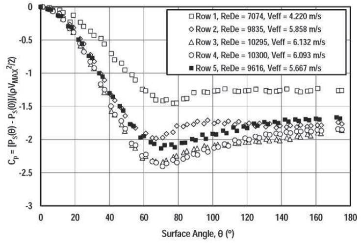
The pins were fabricated from clear acrylic. The midspan surface static pressure distributions were acquired using a 2.54 cm diameter pin which contained 20 equally spaced 0.76 mm static pressure taps around the midspan perimeter. Measurements were made in 6° increments by indexing the pin. An example of pressure distribution is given in figure 6.

Figure 6 : Midline pressure coefficient distribution, rows 1-5, $Re_{D}=100000$ (image taken from Ames et al. (2005))

Pin fin array turbulence and velocity measurements

Array turbulence and velocity measurements were acquired using single and X wire hotwire probes powered by a TSI IFA 300 constant temperature anemometry unit. A special low velocity jet was developed to calibrate the wires from 0.4 m/s through 40 m/s to enable measurements of turbulence and velocity distributions over a 10 to 1 range in Reynolds number. An example of mean and r.m.s. stream-wise velocity component profiles obtained along line B (specified in figure 9) for row 5 is given in figure 7 for the three Reynolds numbers.

Figure 7 : Mean and r.m.s. stream-wise velocity component along line B for different Reynolds numbers - row 5 (image taken from Ames et al. (2006))

Endwall heat transfer measurements

Full surface endwall heat transfer measurements were acquired using a constant heat flux test surface and a FLIR SC500 IR camera. A constant surface heat flux boundary condition was generated using three, 15.28 cm wide by 68.58 cm long, 0.023 mm thick Inconel foils with 0.127 mm thick Kapton backing and 0.05 mm thick acrylic adhesive. The three foils were adhered to a 0.89 mm thick sheet of fiberglass epoxy board which in turn was epoxied to a 3.81 cm thick section of isocyanurate foam. The three foils were connected in series. The current through the foil and the voltage across the center foil was used to determine the surface heat flux. The surface heat flux was corrected for both local radiation and conduction loss. The radiation loss assumed that the emissivity of the surface was 0.96 and the conduction loss was based on a simple 1-D model. The camera was equipped with a special lens which allowed a much wider angle (45°) and a much closer focal plane (6.35 cm) than the standard lens. This allowed the camera to acquire a 130 by 260 pixel image (3.175 cm by 6.35 cm) through a 5.08 cm diameter zinc selenide window. At each measurement location, the camera location was indexed on the pins to ensure a consistent camera location for all the measurements. The accuracy of the surface temperature measurement was enhanced by the calibration of the camera on a calibration surface through the same zinc selenide window, the manual resetting of the camera every three or four pictures, and the averaging of 9 images for each heat transfer realization. The driving force temperature difference was calculated as heated endwall surface temperature corrected for the inlet temperature during the test and for the local calibration less the unheated endwall surface temperature corrected for the inlet temperature and the local calibration. The temperature difference also accounted for the bulk temperature rise of the air due to endwall heating.

The normalized Nusselt number obtained in the experiments on the bottom heated wall is shown in figure figure 8.

Figure 8 : The normalized Nusselt number for different Reynolds numbers (image taken from Ames et al. (2007), form top to bottom: $Re_{D}=3000$, $Re_{D}=10000$, $Re_{D}=10000$.

Data uncertainties

Uncertainties in the reported values were estimated based on the root sum square method described by Moffat (1988). The uncertainty in the reported Reynolds number was determined to be +/- 3% due to the possible error in the flow rate measurement. The largest uncertainty for the midspan pressure coefficient was estimated to be +/- 0.075 due to the very low dynamic pressure at the low Reynolds number condition (Re = 3 000). However, the uncertainty in the pressure coefficient was no more than +/- 0.025 at the higher two Reynolds numbers. Uncertainty in the measurement of velocity using a hot wire was estimated to be +/- 3% except in the near wall region where positional and conduction effects could substantially increase the possible error. Additionally, at high turbulence levels, single wire velocities can be significantly overestimated if transverse fluctuation velocities, normal to the wire become high. For example, at 30% intensity levels, velocities can be overestimated by 4%. The reported value of turbulence intensity had an uncertainty of approximately +/- 3%. The reported uncertainties in the local Nusselt number are estimated to be equal to +/- 12%, +/-11.4%, and +/-10.5% for the 3 000, 10 000, and 30 000 Reynolds numbers, respectively, in the endwall regions adjacent to the pins and +/- 9% away from the pin. Note that the combination of several methods reduced the uncertainty band of the surface temperature measurement from about +/-2 °C to about +/- 0.7 °C. Uncertainty estimates were determined using a 95% confidence interval.

Experimental results used for the CFD evaluation

In the last section, with figures taken directly from the experimental papers, the coordinate system is as usual in these papers, i.e. Z being spanwise and Y vertical. In the computations, these coordinates were switched and this coordinate system is used from here on (see figure 9), i.e. Y is spanwise and Z vertical.

All 1-D profiles are drawn along lines A1, B & C (see Figure 9). The main lines for the velocity components and the Reynolds stresses are A1 and B and the main one for the pressure coefficient is C (mid-span location). Note that

• the experimental results (mean and r.m.s. velocities) on line A1 have been only measured near the bottom wall so that the profiles do not extend to the region near the upper wall,
• the experimental results (mean and r.m.s. velocities) on line B have been only measured near one pin wall so that the profiles do not extend to the region near the opposing pin wall,
• the pressure coefficient along line C is given for an angle between 0° and 180°.

The exact positions of the lines are the following (see Figure 9):

• A1- Line at mid-span location (Y/D=5/4 from center of the pin or Y/D=3/4 from surface of the pin) between two adjacent pins of the same row along the channel height (Z-axis).
• B - Surface to surface line between two adjacent pins of the same row at mid height (Z/D=1.0) along the span (Y-axis).
• C - Circumferential line around the pin surface from 0°-180°, at mid height of the pin (Z/D=1.0). Angle measurements are taken to be zero (0°) on the leading edge of the pins with a counter-clockwise orientation.

Data will be shown for several rows, mainly X/D=0 (row 1), X/D=2.5 (row 2), X/D=5.0 (row 3), and X/D=10.5 (row 5). Note that profiles along line A1 will be shown only for $Re_{D}=30000$.

The velocity components and the Reynolds stresses will be normalized by the average gap bulk velocity $V_{BG}$. If $V_{0}$ stands for the bulk velocity at the inlet, one has, thanks to the mass conservation, $V_{BG}=P/(P-D)V_{0}$.

As the wall heat flux $q_{w}$ is imposed, the Nusselt number is given by $Nu=q_{w}D/(\lambda (T_{w}-T_{ref}))$ where $T_{w}$ and $T_{ref}$ are respectively the time average temperature at the wall and a reference temperature and $\lambda$ is the thermal conductivity. $T_{ref}$ takes into account the increase in the bulk temperature of the fluid from the heated surface as it flows down the array (see the Nusselt number calculated in Nordquist (2006)).

Then, at a given $X$, one has: $T_{ref}=q_{w}S_{h}(X)/(\rho C_{p}V_{0}S_{i})$.

Where $S_{h}(X)$ is the heated surface from the inlet to $X$. Nordquist (2006) uses an estimation of this surface using $S_{h}=(-X_{inlet}+X)S_{htot}/L_{X}$ where $X_{inlet}$ in the X coordinate of the inlet plane, $S_{htot}$ the total heated surface (here the surface from $X_{inlet}$ to $X_{outlet}$) and $L_{X}$ the total length of the domain ($L_{X}=X_{outlet}-X_{inlet}$). $\rho$, $C_{p}$ and $S_{i}$ are the fluid density, the specific heat and the surface inlet, respectively.

The following data will be analyzed for the different computations:

• The pressure loss coefficient $f=\Delta P/(2\rho {V^{2}}_{BG}N_{rows})$ where $\Delta P$ is the pressure drop between the planes X/D=-5 and X/D=22.5 and $N_{rows}$ the number of rows ($N_{rows}=8$ in the present case). The experimental values can be found in File:Headloss.xls.
• The pressure coefficient along line C for rows 1, 2, 3 and 5. $C_{p}=2(p-p_{max})/\rho {V^{2}}_{BG}$ where $p_{max}$ is the maximum pressure (the pressure at the stagnation point). The experimental data can be found in File:Cp midline.zip.
• The normalized mean stream-wise velocity ($U/V_{BG}$) and its r.m.s value ($u'/V_{BG}$) along lines A1 and B.

The experimental data can be found in File:Dynamics.zip.

• $Nu_{av}$, the average of the Nusselt number on the bottom wall between X/D=-2.5 and X/D=20. The experimental values can be found in File:Nusselt average.xls.
• The normalized Nusselt number ($Nu/Nu_{av}$) on the bottom wall. The experimental data can be found in File:Thermal Fields bottom wall.zip.
• The normalized Nusselt number profile along two specified lines $Y=0$ and $Y=1.25D$ (see figure 10) if one considers the computational domain global frame, see figure 11). Note that one can extract other lines for comparisons from the file File:Thermal Fields bottom wall.zip.

Figure 9 : Rows numbering and lines (A1, B and C) locations. i=1,..,8. Line C : Centerline of the cylinder (Z=D), 0° at the impingement (rotation sense : counter clockwise with Z axis from bottom to top wall), line A1: X=2.5D (i-1), Y=0 if i is even and Y=1.25D if i is odd, 0 ≤ Z ≤ 2D, line B: X=2.5D (i-1), -0.75D ≤ Y ≤ 0.75D if i is even and 0.5D ≤ Y ≤ 2D if i is odd, Z=D.

Figure 10 : The lines along which the normalized Nusselt number are plotted

CFD Methods

The computational domain

The following computational domain, which has been chosen for the 15th Ercoftac workshop, is a subdomain of the experimental flow domain assuming lateral periodicity. It consists of 8 by 2 pins (see figure 11). This assumption reduces possible periodicity effects while keeping reasonable grid sizes. All solid surfaces (pins, bottom and top walls) are set to no-slip solid walls. The inlet of the channel is set at a distance $L_{U}=10D$ upstream from the center of the first row of pins, whereas the outlet is $L_{D}=15D$ downstream from the center of the last row of pins (this gives $X_{inlet}=-10D$ and $X_{outlet}=32.5D$), respectively. Note that these two distances are both equal to 7.75D in the experimental setup but are not enough to perform reliable CFD calculations (see Afgan et al. (2007) and Parnaudeau et al. (2008)), in particular for the upstream channel, unless one represents the nozzle of the experiment (see figure 5) what will lead to much more expensive computations.

The main computational results submitted for the workshop were the EDF R&D computations, and these will be presented here.

Figure 11: The computational domain (the global frame is indicated in red in the figure)

General Description of the computations

All the computations presented herein have been carried out with Code_Saturne (see Archambeau et al. (2004)), an EDF in-house open source CFD tool for incompressible flows (go to http://code-saturne.org for more details and download). It is based on an unstructured collocated finite-volume approach for cells of any shape (here only hexa conforming meshes are used). It uses a predictor/corrector method with Rhie and Chow interpolation and a SIMPLE-like algorithm for pressure correction. An implicit reconstruction method is used for the gradients while dealing with the non-orthogonalities.

Four Models, LES using the dynamic subgrid-scale model (Germano et al. (1991), Lilly (1992)) and URANS using kω-SST (Menter (1994)), φ-model (Laurence et al. (2005)), and EB-RSM (Manceau and Hanjalic (2002)) are used to simulate the present test-case (the main computations and results have been presented in Benhamadouche et al. (2012)). All the models are wall-resolved and use no-slip boundary conditions for the velocity vector and appropriate boundary conditions for the turbulent quantities (see the corresponding articles). Three Reynolds numbers have been computed: $Re_{D}=3,000$, $Re_{D}=10,000$ and $Re_{D}=30,000$. The latter is computed only with URANS approaches and the first one only with LES.

Inlet conditions for the velocity and turbulent quantities will be specified separately for the LES and URANS computations. No sensistivity tests concerning the boundary conditions are reported.

The temperature is treated as a passive scalar with an imposed temperature at the inlet, an imposed heat flux at the bottom wall and adiabatic conditions elsewhere. The effect of the thermal boundary condition on the bottom wall is studied in LES by taking a fixed temperature instead of a fixed heat flux.

Practically, the density, the inlet velocity, the specific heat coefficient and the diameter of the pins are set equal to unity and the viscosity equal to $1/Re_{D}$. The Prandtl number is equal to 0.71 and thus the fluid conductivity $\lambda =1/(PrRe_{D})$. As the temperature is passive, the inlet temperature is taken equal to 0 and the imposed heat flux equal to unity.

Zero-gradient boundary conditions are used for all the variables at the outlet and an implicit periodic condition is used in the lateral direction for all the variables.

Although only the non dimensional parameters are of importance (here the Reynolds and Prandtl numbers), in order to mimic the experiment with physical values, table 1 provides typical values which might be used for the simulations (the pressure is equal to the atmospheric pressure and the computation is incompressible).

All the computations have been run on EDF BlueGene/P and BlueGene/Q using up to 4096 cores for LES computations.

Table 1: typical values that can be used in a computation

$Re_{D}$	$T_{inlet}$ (°K)	$V_{0}$ (m/s)	$\nu$ (m²/s)	$\rho$ (kg/m^3)	$C_{p}$ (J/kg/K)	$\lambda$ (W/m/K)	$q$ (W/m²)
3000	300	1.06	0.000015	1.2	1005	0.0255	100
10000	300	3.54	0.000015	1.2	1005	0.0255	300
30000	300	10.62	0.000015	1.2	1005	0.0255	1000

Computational meshes

The meshes used for LES and URANS computations are of the same kind and have been created with Gambit. Figure 12 shows top and side view of the mesh used for LES at $Re_{D}=3000$. The main parameters for meshing the pins are given in table 2 for the different computations. $nb$, $nb_{\theta }$ and $nb_{z}$ give the cell numbers in the computational domain, around a pin and between the top and bottom walls, respectively. $\Delta n_{\theta }$ and $\Delta n_{z}$ are the wall cell size in the wall normal direction around the pins and at the top and bottom walls, respectively. $\Delta Y$ is the cell size in the mid-plane($Z=D$) in Y direction.

Note that for URANS, only the parameters used for the finest grid are mentioned. The two coarser levels are obtained by coarserning the grid spacings by 2 in all the directions. This has been done for convergence study purposes but could have been optimized (the finest meshes in URANS contain 17 million and 29 million cells at $Re_{D}=10000$ and $Re_{D}=30000$, respectively, and this could have been clearly reduced in order to obtain a converged Unsteady RANS solution).

Table 2: Mesh information

Computation	$nb$	$nb_{\theta }$	$nb_{z}$	$\Delta n_{\theta }/D$	$\Delta n_{z}/D$	$\Delta n_{zh}/D$
LES $Re_{D}=3000$	18.2 million	176	90	0.0028	0.0065	0.0536
LES $Re_{D}=10000$	76.2 million	320	120	0.0015	0.0019	0.0584
URANS(*) $Re_{D}=10000$	17 million	128	112	0.00075	0.001	0.065
URANS(*) $Re_{D}=30000$	29 million	128	160	0.00025	0.00025	0.0625

(*) Only the information of the finest mesh are given. The two coarser levels of refinement are obtained by coarserning the grid spacings by 2 in all the directions

Figure 12: Cuts of the computational mesh (LES at $Re_{D}=3,000$). Top: top view showing the duplicated pattern, Bottom: side view

Large Eddy Simulation Computations

General Features

Large Eddy Simulation (see Benhamadouche (2006) for its implementation in Code_Saturne) uses a dynamic Smagorinsky model (Germano et al. (1991), Lilly (1992)) in which the Smagorinsky constant cannot be negative and is bounded by its value validated in a channel flow ($C_{S}=0.065$). This model has been successfully used recently by Afgan et al. (2011) for the flow around a single cylinder and around two side-by-side cylinders. A fully centered convection scheme is applied for the velocity components and the temperature. For the latter, a slope test which switches to a first order upwind scheme is utilized to limit the overshoots. The time advancing scheme is second order based on a Crank-Nicolson/Adams Bashforth scheme (the diffusion including the velocity gradient is totally implicit, the convection is semi-implicit and the diffusion including the transpose of the velocity gradient is explicit). A turbulent Prandtl number equal to 0.5 is used when solving for the temperature with LES.

At the inlet, a uniform velocity is imposed without any synthetic or precursor turbulence generation. Note that the reported turbulence intensity in the experiment is about 1.4% which would be difficult to impose. In fact, inlet conditions will certainly affect the flow around the first row and probably around the second one but not around the next ones.

Very fine wall-resolved LES simulations have been carried out for the Reynolds numbers $Re_{D}=3,000$ and $Re_{D}=10,000$.

Wall treatment in LES

Particular attention has been paid to the grid refinement at the wall. Two meshes containing 18 million and 76 million cells have been utilized to simulate the two Reynolds numbers $Re_{D}=3,000$ and $Re_{D}=10,000$, respectively. Figures 13 and 14 show, for the two test-cases, instantenous snapshots of the non-dimensional wall normal distances of the first computational cells center to the wall. $\Delta n$ is the half wall normal mesh size of near wall computational cells and ${\Delta n}^{+}$ the corresponding value made dimensionless with the local friction velocity. The two meshes are of the same quality for this quantity (the maximum value is higher for $Re_{D}=10,000$ but this is rather a local effect).

${\Delta n}^{+}$ is not the only quantity of interest; one has to have a reasonably fine mesh also in the stream-wise and span-wise directions. Figure 15 gives, for LES computation at $Re_{D}=10,000$, an overview of the mean non-dimensional grid spacings in the wall normal direction (${\Delta n}^{+}$), in the direction parallel the tangential mean velocity at the first computational cell (${\Delta \tau _{x}}^{+}$) and in the direction normal to the plane (${n}$,${\tau _{x}}$) (${\Delta \tau _{z}}^{+}$). It can be seen that the refinement is the one needed for a wall resolved LES everywhere except around the centerlines of the pins and downstream of the last row. However, the refinement in these regions is still very satisfactory.

Figure 13: Instantaneous snapshots of ${\Delta n}^{+}$, the non-dimensional half wall normal mesh size of near wall computational cells, LES at $Re_{D}=3,000$ with 18 million computational cells

Figure 14: Instantaneous snapshots of ${\Delta n}^{+}$, the non-dimensional half wall normal mesh size of near wall computational cells, LES at $Re_{D}=10,000$ with 18 million computational cells

Figure 15: Mean non-dimensional grid spacings of the near-wall computational cell, LES at $Re_{D}=10,000$ with 76 million computational cells - top left: ${\Delta \tau _{x}}^{+}$ - top right: ${\Delta \tau _{z}}^{+}$ - bottom: ${\Delta n}^{+}$

Sensitivity to the sub-grid scale model

Calculations have been carried out also without using a subgrid-scale model in order to quantify the effect of this model. They showed that the effect is not that important at the present level of refinement. Figures 16 and 17 show profiles of the r.m.s. values of the stream-wise velocity component and of the normalized Nusselt numbers, respectively. The effect seems almost negligible.

Table 3 gives the pressure loss coefficient and the averaged Nusselt number for the simulations with and without the sub-grid scale model. Although the sub-grid scale model has almost no influence on the pressure drop coefficient, one can see that there is a slight effect on heat transfer which has not been seen locally (as the global Nusselt number is averaged over the bottom wall). The effects are, however, small and one can argue that the meshes are fine enough. Note that only first and the second order moments have been considered for comparison. There is no doubt one could see effects on the resolved dissipation rate or higher order statistics.

Figure 16: R.m.s. of the stream-wise velocity component along line B - effect of the sub-grid scale model on LES at $Re_{D}=3000$

Figure 17: Local Nusselt number on the bottom wall - effect of the sub-grid scale model on LES at $Re_{D}=3000$

Table 3: Effect of sub-grid scale model on the global quantities

	With a sub-grid scale model (dynamic)	Without a sub-grid scale model
Pressure Loss coefficient (f)	0.1076	0.1089
Error on f (%)	3	2
Averaged Nusselt Number ($Nus_{av}$)	21.6	20.8
Error on $Nus_{av}$ (%)	2	6

URANS computations

General Features

Three URANS approaches are utilized: the kω-SST model (Menter (1994)), the φ-model (Laurence et al. (2005)) and the EB-RSM model (Manceau and Hanjalic (2002)). All the models are wall-resolved (Low Reynolds Number models).

The kω-SST uses a blending between the k-ω and the standard k-ε. The φ-model uses the elliptic relaxation concept introduced by Durbin (1991). Originally, Durbin proposed (v²-f model, Durbin (1995)) to solve two more equations in addition to the k and ε equations: a transport equation for v² and an elliptic equation for the redistribution term. Unfortunately, the boundary conditions proposed originally were too stiff. The φ-model proposes a more stable formulation using a change of variable (v²/k). Then, v² is used in the definition of the eddy viscosity. In both utilized eddy viscosity models, a Simple Gradient Diffusion Hypothesis (SGDH) is utilized for the temperature equation with a turbulent Prantl number equal to 0.9.

The EB-RSM model is presented in Manceau and Hanjalic (2002). It is inspired by the elliptic relaxation concept for the Reynolds stresses. Instead of proposing six relaxation equations, it proposes to solve one elliptic equation for a parameter α which is equal to zero at the wall and goes to 1 in the homogeneous region. Then, this parameter is used to blend the scrambling and the dissipation terms of the Reynolds stresses between the near wall region and the homogeneous one. It uses for example the Speziale, Sarkar and Gatski model (SSG model (1991)) for the homogeneous part of the scrambling term. In the EB-RSM model, the temperature equation is solved with a Generalized Gradient Diffusion Hypothesis (GGDH) approach using a constant equal to 0.23. The use of more advanced models such us the AFM (Algebraic Flux Model), the EB-GGDH (extension of the elliptic blending concept but for the scrambling and dissipation terms of the turbulent heat fluxes (see Dehoux et al. (2012) for more details)) or the EB-AFM didn't change the results that much, at least for global quantities such as the mean Nusselt number.

When using URANS, a uniform velocity and 5% turbulence intensity are imposed at the inflow. Putting 0% turbulence made the computations degenerate towards Q-DNS (the modelled turbulent kinetic energy or Reynolds stresses vanished). After some tests, it has been found that 5% turbulence is a good compromise (1% was not enough). Note that inlet conditions will certainly affect the flow around the first row and probably around the second one but not around the next ones.

The inlet conditions for URANS computations are thus given by:

The turbulent kinetic energy $k$ is given by:

$k={\frac {3}{2}}V_{BG}^{2}I_{k}^{2}$

where $V_{BG}$ is the average gap bulk velocity and $I_{k}$ the turbulent intensity.

In the case of the Reynolds stress model, the Reynolds stresses are given by:
$R_{ij}={\frac {2}{3}}k\delta _{ij}$

The turbulent dissipation $\varepsilon$ is given by:
$\varepsilon ={\frac {C_{\mu }^{3/4}k^{3/2}}{0.1\kappa D_{H}}}$

where $\kappa =0,42$, $C_{\mu }=0.09$ and $D_{H}=2H$ stands for the hydraulic diameter of the inlet.

In the case of the kω-SST model, one takes $\omega ={\frac {\varepsilon }{C_{\mu }k}}$.

URANS simulations have been carried out with the three models for the two higher Reynolds numbers; $Re_{D}=10,000$ and $Re_{D}=30,000$.

By default, a centered scheme with a slope test is used for the velocity components and the temperature and a 1st order upwind scheme for the turbulent quantities. The time advancing scheme is in this case a first order Euler one. As shown below for the EB-RSM model, a systematic sensitivity study with respect to the mesh refinement and to the numerical options has been carried out in order to have a high confidence in the computations.

Grid convergence study

The grid convergence study has been performed for the three URANS models and for the two higher Reynolds numbers. As eddy viscosity and Reynolds stress models exhibited totally different behaviors, the sensitivity study has been carried out for all the models. Hereafter, the study performed for $Re_{D}=10,000$ and the EB-RSM model is presented. Three levels of refinement are used for all the models. The coarse mesh is successively refined by a factor 2 in the three directions. The finest mesh has approximately 17M cells for $Re_{D}=10,000$ (it contains approximately 29M cells for $Re_{D}=30,000$).

Figures 18, 19 and 20 show the pressure coefficient along the pin midline and the mean and r.m.s. values of the stream-wise velocity component along line B. As the computations are unsteady, note that the r.m.s. values, or more generally the Reynolds stresses, are the sum of the resolved part and the modelled part: $R_{ij}=R_{ij}^{res}+R_{ij}^{mod}$. The resolved and modeled part are shown separately in figures 21 and 22. Note that the summing does not apply to the rms values but to the actual stresses and then one takes the square root for the diagonal quantities.

One can observe that the results of the two finer meshes do not quite match, the coarse mesh results being very far from the actual ones. Thus, all the results given in "Evaluation" for a turbulence model will be those obtained with the finest mesh (called here "very fine mesh"). The ideal would have been to add a fourth level of refinement but this would have expensive in terms of CPU time. Note also that the refinements could have been "more intelligent" than refining by a factor of 2 in all the directions. However, the sensitivity study on the numerical options (see next section) make us confident that the results obtained with the finest mesh are very close to the converged ones.

Figure 18: Mean pressure coefficient along the pin midline, EB-RSM at $Re_{D}=10,000$ - grid convergence study

Figure 19: Mean stream-wise velocity component along line B, EB-RSM at $Re_{D}=10,000$ - grid convergence study

Figure 20: R.m.s. of the stream-wise velocity component along line B, EB-RSM at $Re_{D}=10,000$ - grid convergence study

Figure 21: Modelled r.m.s. of the stream-wise velocity component along line B, EB-RSM at $Re_{D}=10,000$ - grid convergence study

Figure 22: Resolved r.m.s. of the stream-wise velocity component along line B, EB-RSM at $Re_{D}=10,000$ - grid convergence study

Sensitivity study to the convection scheme

By default, a centered scheme with a slope test is used for the velocity components and the temperature and a 1st order upwind scheme for the turbulent quantities. The scheme called centered in figures 23 and 24 consists of a fully centered scheme for the velocity components and a centered scheme for all the other scalar quantities (Reynolds stresses, dissipation rate, temperature). As it can be observed, the effect is everywhere negligible on the mean and r.m.s. quantities except around row 3 where it is noticeable but limited. This conclusion is important as a pure centered scheme on the velocity components doesn't seem to change the unsteadiness. Moreover, using a centered scheme for the turbulent quantities doesn't affect the results. Other tests have been carried out by introducing for example outer iteration for pressure/velocity coupling and none of them exhibited a noticeable effect.

Figure 23: Mean stream-wise velocity component along line B, EB-RSM at $Re_{D}=10,000$ - sensitivity study to the numerical scheme on the very fine mesh

Figure 24: r.m.s. of the stream-wise velocity component along line B, EB-RSM at $Re_{D}=10,000$ - sensitivity study to the numerical scheme on the very fine mesh

The main computations

Table 4 summerizes the main computations which will be exhibited in "Evaluation". Note that "niba = number of iterations before averaging" and "nifa = number of iterations for averaging".

Table 4: The main computation which are used in the evaluation part

	Test-case	$Re_{D}$	$V_{BG}$ (m/s)	$V_{B}$ (m/s)	Turbulence Model	Time step (s)	niba	nifa	mean $CFL_{max}$
LES3000	3000	2.02	1.21	Dynamic Smagorinsky	0.0015	325000	217000	0.8
LES10000	10000	6.18	3.71	Dynamic Smagorinsky	0.0002	130000	245000	0.8
EBRSM10000	10000	6.18	3.71	EB-RSM	0.001	160000	140000	1.8
PHI10000	10000	6.18	3.71	φ-model	0.001	50000	250000 (*)	1
kwSST10000	10000	6.18	3.71	kω-SST	0.001	80000	220000 (*)	1.3
EBRSM30000	30000	18.53	11.12	EB-RSM	0.0000625	64000	308000	0.6
PHI30000	30000	18.53	11.12	φ-model	0.00025	40000	125000	0.9
kwSST30000	30000	18.53	11.12	kω-SST	0.00025	50000	150000	1.8

(*) 100000 would have been enough to converge in time

Possible sources of uncertainty

The main possible sources of uncertainty are:

• The inflow conditions
• The periodicity assumption in the spanwise direction.
• The uniformity of the heat flux which is probably not the case in the experiment.

---

Contributed by: Sofiane Benhamadouche — EDF

Front Page

Description

Test Case Studies

Evaluation

Best Practice Advice

References

© copyright ERCOFTAC 2024