UFR 4-18 Test Case

Flow and heat transfer in a pin-fin array

Front Page

Description

Test Case Studies

Evaluation

Best Practice Advice

References

Test Case Study

Brief Description of the Study Test Case

This should:

• Convey the general set up of the test-case configuration( e.g. airflow over a bump on the floor of a wind tunnel)
• Describe the geometry, illustrated with a sketch
• Specify the flow parameters which define the flow regime (e.g. Reynolds number, Rayleigh number, angle of incidence etc.)
• Give the principal measured quantities (i.e. assessment quantities) by which the success or failure of CFD calculations are to be judged. These quantities should include global parameters but also the distributions of mean and turbulence quantities.

The description can be kept fairly short if a link can be made to a data base where details are given. For other cases a more detailed, fully self-contained description should be provided.

The experiments from Ames et al. deal with the flow of air around 8 staggered rows of 7.5 heated pins, spaced at P=2.5D in both stream-wise and span-wise directions (based on center to center distances). The diameter of the pins is set to 0.0254 m (1 inch) and the channel height is twice the diameter (H=2D). The Reynolds numbers $Re_{D}$ based on the pin diameter and the average gap bulk velocity which have been tested are equal to 3,000, 10,000 and 30,000, respectively. The gap bulk velocity is determined between two adjacent pins of the same row. Taking $V_{0}$ and $V_{G}$ as the inlet and gap velocities, respectively, and considering mass conservation, one obtains $V_{G}=P/(P-D)V_{0}$.

A sketch of the original experimental configuration is given in Figure 1. In the experiment, the distance between the inlet (beginning of the test section; end of a converging nozzle) and the center of the first cylinders is equal to 7.75D. The distance between the center of the last cylinders and the test section is also equal to 7.75D.

The bottom wall is heated with a constant heat-flux whereas the other walls are adiabatic (Ames et al.). All the flow properties can be taken constant, the Prantl number is equal to 0.71.

Figure 1: Sketch of Ames et al. experiment

Test Case Experiments

Provide a brief description of the test facility, together with the measurement techniques used. Indicate what quantities were measured and where.

Discuss the quality of the data and the accuracy of the measurements. It is recognized that the depth and extent of this discussion is dependent upon the amount and quality of information provided in the source documents. However, it should seek to address:

• How close is the flow to the target/design flow (e.g. if the flow is supposed to be two-dimensional, how well is this condition satisfied)?

• Estimation of the accuracy of measured quantities arising from given measurement technique

• Checks on global conservation of physically conserved quantities, momentum, energy etc.

• Consistency in the measurements of different quantities.

Discuss how well conditions at boundaries of the flow such as inflow, outflow, walls, far fields, free surface are provided or could be reasonably estimated in order to facilitate CFD calculations

General Description

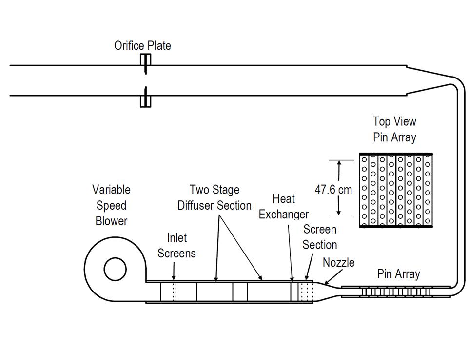
The description given in the present section has been given by F. Ames during the $15^{th}$ Ercoftac SIG15 Workshop. More information could also be found in Ames et al. (2004, 2005, 2006, 2007). The objective of the experiments was to create a database that includes heat transfer distributions on the pin fins and endwall, pressure distributions on the pin fins and endwall, documentation of turbulence intensities and scales, and measurements of turbulence and velocity distributions across the channels. The research was conducted in a small bench top wind tunnel (see Figure 2) which included a small blower capable of producing a flow of $0.3m^{3}/s$ at a static pressure rise of 2000 Pa. The pin fin array was designed in an 8 row, 7 1/2 pin per row staggered arrangement. Both the cross passage (S/D) and stream-wise (X/D) pin spacing were equal to 2.5 while the pin height to diameter (H/D) was 2. The pin diameter was chosen to be equal to 2.54 cm. The flow conditioning system first spreads out the flow from the blower to the width of the array using a two-stage multi-vane diffuser. A heat exchanger was installed in the system downstream from the diffuser to control the tunnel temperature in order to impose a constant value. The heat exchanger discharges the flow into a screen box consisting of three nylon window screens to reduce the cross stream velocity variations in the flow. Directly downstream of the screens, the flow enters a smooth 2.5 to 1 area ratio nozzle prior to entering the test section. The pin fin array test section begins 7.75 D upstream of the centerline of the first row of pins and ended 7.75 D downstream of the centerline of the last row of pins. The inlet total temperature and pressure and static pressures were measured 5 D upstream from the row 1 centerline and the exit static pressures were measured 5 D downstream from row 8. Downstream from the test section the flow was directed through a 90° rectangular elbow then a rectangular channel followed by a second 90° elbow before entering a 20.8 cm diameter orifice tube used to measure the array flow rate. Tests were conducted at three Reynolds numbers : 3 000, 10 000, and 30 000. The Reynolds number is based on the maximum velocity (also called the gap velocity $V_{G}$, see the previous section). Fluid properties were determined from the inlet conditions.

The remaining description will focus on the data which are used in the present work, the heat transfer on the pins, the pressure distributions on the endwalls, availabe spectra ... are not included.

Figure 2: Sketch of Ames et al. experimental rig (image taken from Ames et al. (2007))

Pin fin surface static pressure

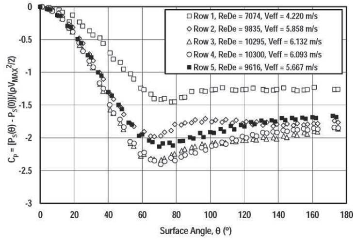
The pins were fabricated from clear acrylic. The midspan surface static pressure distributions were acquired using a 2.54 cm diameter pin which contained 20 equally spaced 0.76 mm static pressure taps around the midspan perimeter. Measurements were made in 6° increments by indexing the pin. An example of pressure distribution is given in figure 3.

Figure 3 : Midline pressure coefficient distribution, row 1-5, Re=10 0000 (image taken from Ames et al. (2005))

Pin fin array turbulence and velocity measurements

Array turbulence and velocity measurements were acquired using single and X wire hotwire probes powered by a TSI IFA 300 constant temperature anemometry unit. A special low velocity jet was developed to calibrate the wires from 0.4 m/s through 40 m/s to enable measurements of turbulence and velocity distributions over a 10 to 1 range in Reynolds number. An example of profile obtained along the line B1 for row 5 is given in figure 4

Figure 4 : Mean and r.m.s. stream-wise velocity component along line B for different Reynolds numbers - row 5 (image taken from Ames et al. (2006))

Endwall heat transfer measurements

Full surface endwall heat transfer measurements were acquired using a constant heat flux test surface and a FLIR SC500 IR camera. A constant surface heat flux boundary condition was generated using three, 15.28 cm wide by 68.58 cm long, 0.023 mm thick Inconel foils with 0.127 mm thick Kapton backing and 0.05 mm thick acrylic adhesive. The three foils were adhered to a 0.89 mm thick sheet of fiberglass epoxy board which in turn was epoxied to a 3.81 cm thick section of isocyanurate foam. The three foils were connected in series. The current through the foil and the voltage across the center foil was used to determine the surface heat flux. The surface heat flux was corrected for both local radiation and conduction loss. The radiation loss assumed the emissivity of the surface was 0.96 and the conduction loss was based on a simple 1-D model. The camera was equipped with a special lens which allowed a much wider angle (45°) and a much closer focal plane (6.35 cm) than the tandard lens. This allowed the camera to acquire a 130 by 260 pixel image (3.175 cm by 6.35 cm) through a 5.08 cm diameter zinc selenide window. At each measurement location, the camera location was indexed on the pins to ensure a consistent camera location for all the measurements. The accuracy of the surface temperature measurement was enhanced by the calibration of the camera on a calibration surface through the same zinc selenide window, the manual resetting of the camera every three or four pictures, and the averaging of 9 images for each heat transfer realization. The driving force temperature difference was calculated as heated endwall surface temperature corrected for the inlet temperature during the test and for the local calibration less the unheated endwall surface temperature corrected for the inlet temperature and the local calibration. The temperature difference also accounted for the bulk temperature rise of the air due to endwall heating.

Figure 5 : The normalized Nusselt number for different Reynolds numbers (image taken from Ames et al. (2007))

Data uncertainties

Uncertainties in the reported values were estimated based on the root sum square method described by Moffat (1988). The uncertainty in the reported Reynolds number was determined to be +/- 3% due to the possible error in the flow rate measurement. The largest uncertainty for the midspan pressure coefficient was estimated to be +/- 0.075 due to the very low dynamic pressure at the low Reynolds number condition (Re = 3 000). However, the uncertainty in the pressure coefficient was no more than +/- 0.025 at the higher two Reynolds numbers. Uncertainty in the measurement of velocity using a hot wire was estimated to be +/- 3% except in the near wall region where positional and conduction effects could substantially increase the possible error. Additionally, at high turbulence levels single wire velocities can be significantly overestimated if traverse fluctuation velocities, normal to the wire become high. For example at 30% intensity levels velocities can be overestimated by 4%. The reported value of turbulence intensity had an uncertainty of approximately +/- 3%. The reported uncertainties in Nusselt number are estimated to be as high at +/- 12%, +/-11.4%, and +/-10.5% for the 3 000, 10 000, and 30 000 Reynolds numbers respectively in the endwall regions adjacent to the pins and +/- 9% away from the pin. Note that the combination of several methods reduced the uncertainty band of the surface temperature measurement from about +/-2 °C to about +/- 0.7 °C. Uncertainty estimates were determined using a 95% confidence interval.

CFD Methods

Provide an overview of the methods used to analyze the test case. This should describe the codes employed together with the turbulence/physical models examined; the models need not be described in detail if good references are available but the treatment used at the walls should explained. Comment on how well the boundary conditions used replicate the conditions in the test rig, e.g. inflow conditions based on measured data at the rig measurement station or reconstructed based on well-defined estimates and assumptions.

Discuss the quality and accuracy of the CFD calculations. As before, it is recognized that the depth and extent of this discussion is dependent upon the amount and quality of information provided in the source documents. However the following points should be addressed:

• What numerical procedures were used (discretisation scheme and solver)?

• What grid resolution was used? Were grid sensitivity studies carried out?

• Did any of the analyses check or demonstrate numerical accuracy?

• Were sensitivity tests carried out to explore the effect of uncertainties in boundary conditions?

• If separate calculations of the assessment parameters using the same physical model have been performed and reported, do they agree with one another?

---

Contributed by: Sofiane Benhamadouche — EDF

Front Page

Description

Test Case Studies

Evaluation

Best Practice Advice

References

© copyright ERCOFTAC 2024