UFR 4-16 Test Case: Difference between revisions
| (309 intermediate revisions by 2 users not shown) | |||
| Line 1: | Line 1: | ||
= Flow in a 3D diffuser = | = Flow in a 3D diffuser = | ||
{{UFRHeader | {{UFRHeader | ||
| Line 64: | Line 63: | ||
resolution of 0.4 x 0.4 x 0.4 mm. Interested readers are referred to | resolution of 0.4 x 0.4 x 0.4 mm. Interested readers are referred to | ||
[[UFR_4-16_References#7|Cherry ''et al.'' (2008]], | [[UFR_4-16_References#7|Cherry ''et al.'' (2008]], | ||
[[UFR_4-16_References# | [[UFR_4-16_References#8|2009)]] | ||
for more details about the measurement technique. | for more details about the measurement technique. | ||
| Line 81: | Line 80: | ||
<div id="figure6"></div> | <div id="figure6"></div> | ||
{|align="center" width="558" | |||
|[[Image:UFR4-16_figure6.jpg|548px]] | |||
|- | |||
|'''Figure 6:''' 3D diffuser arrangement in a medical magnetic resonance imaging device. Courtesy of J. Eaton (Stanford University) | |||
|} | |||
===Mean velocity and Reynolds stress measurements=== | |||
Cherry ''et al.'' provided a detailed reference database comprising the | |||
three-component mean velocity field and the streamwise Reynolds stress component | |||
field within the entire diffuser section. Both diffuser configurations | |||
considered are characterized by a three-dimensional boundary-layer | |||
separation, but the slightly different expansion geometries caused the size | |||
and shape of the separation bubble exhibiting a high degree of geometric | |||
sensitivity to the dimensions of the diffuser as illustrated in | |||
[[UFR_4-16_Test_Case#figure7|Figs. 7]], [[UFR_4-16_Test_Case#figure8|8]] | |||
and [[UFR_4-16_Test_Case#figure9|9]] | |||
<div id="figure7"></div> | |||
{|align="center" width="750" | |||
|[[Image:UFR4-16_figure7.png|740px]] | |||
|- | |||
|'''Figure 7:''' Streamwise velocity contours in a plane parallel to the top wall, from [[UFR_4-16_References#7|Cherry ''et al.'' (2008)]] | |||
|} | |||
<div id="figure8"></div> | |||
{|align="center" width="750" style="border: 1px solid black;" border="1" | |||
|align="center" colspan="3"|[[Image:UFR4-16_figure8a.png|493px]] | |||
|- | |||
|colspan="3"|[[Image:UFR4-16_figure8b.png|750px]] | |||
|- | |||
|[[Image:UFR4-16_figure8c.png|247px]]||[[Image:UFR4-16_figure8d.png|247px]]||[[Image:UFR4-16_figure8e.png|247px]] | |||
|- | |||
|colspan="3"|'''Figure 8:''' Measured streamwise velocity contours in the central plane (upper) of the '''Diffuser 1''' and in the three selected cross-sectional slices positioned at different distances from the diffuser inlet (lower; their locations are denoted by thick white lines in the upper figure). Note that the black line indicates zero streamwise velocity and the purple and pink regions are reverse flow. The velocity values are normalized by the bulk inlet velocity being ''V<sub>ref</sub>=1 m/s''. Courtesy of J. Eaton (Stanford University) | |||
|} | |||
<div id="figure9"></div> | |||
{|align="center" width="750" style="border: 1px solid black" border="1" | |||
|colspan="3" align="center"|[[Image:UFR4-16_fig9a.png|493px]] | |||
|- | |||
|colspan="3"|[[Image:UFR4-16_fig9b.png|750px]] | |||
|- | |||
|valign="bottom"|[[Image:UFR4-16_fig9c.png|246px]] | |||
|valign="bottom"|[[Image:UFR4-16_fig9d.png|246px]] | |||
|valign="bottom"|[[Image:UFR4-16_fig9e.png|246px]] | |||
|- | |||
|colspan="3"|'''Figure 9:''' Measured streamwise velocity contours in the central plane (upper) of the '''Diffuser 2''' and in the three selected cross-sectional slices positioned at different distances from the diffuser inlet (lower; their locations are denoted by thick white lines in the upper figure). Note that the black line indicates zero streamwise velocity and the purple and pink regions are reverse flow. The velocity values are normalized by the bulk inlet velocity being ''V<sub>ref</sub>=1 m/s''. Courtesy of J. Eaton (Stanford University) | |||
|} | |||
<div id="figure10"></div> | |||
{|align="center" width="750" style="border: 1px solid black" | |||
!x/h=2!!x/h=5!!x/h=8!!x/h=12!!x/h=15 | |||
|- | |||
|valign="bottom"|[[Image:UFR4-16_fig10a.png|137px]] | |||
|valign="bottom"|[[Image:UFR4-16_fig10b.png|139px]] | |||
|valign="bottom"|[[Image:UFR4-16_fig10c.png|148px]] | |||
|valign="bottom"|[[Image:UFR4-16_fig10d.png|154px]] | |||
|valign="bottom"|[[Image:UFR4-16_fig10e.png|162px]] | |||
|- | |||
|align="center" colspan="5"|[[Image:UFR4-16_fig10f.png]] | |||
|- | |||
|colspan="5"|'''Figure 10:''' Measurements of turbulent streamwise stress components taken in cross-sectional slices of the diffuser 1 perpendicular to the mean flow. The region of highest turbulence (red areas; ignore the red areas at the bottom walls) follows the shear layer between forward and reverse flow. ''h''=1cm represents the height of the inflow duct. Courtesy of J. Eaton (Stanford University) | |||
|} | |||
===Pressure measurements=== | |||
In addition | |||
[[UFR_4-16_References#8|Cherry ''et al.'' (2009)]] | |||
provided the pressure distribution along | |||
the bottom non-deflected wall of diffuser 1 at different Reynolds numbers. | |||
Complementary to the Reynolds number 10000 (for which the entire flow field | |||
was measured), two higher Reynolds numbers — 20000 and 30000 — were also | |||
considered, [[UFR_4-16_Test_Case#figure11|Fig. 11]]. The surface pressure distribution was evaluated to | |||
yield the coefficient | |||
<math>C_p=(p-p_\textrm{ref})/(0.5\rho U_\textrm{bulk}^2)</math>; | |||
the reference pressure was taken at the | |||
position ''x/L = 0.05''. The pressure curve exhibits a development typical of | |||
flow in diverging ducts. The pressure decrease in the inflow duct is | |||
followed by a steep pressure increase already at the very end of the inflow | |||
duct and especially at the beginning of the diffuser section. The | |||
transition from the initial strong pressure rise to its moderate increase | |||
occurs at ''x/L ≈ 0.3'', (''x/h=4.5'') | |||
corresponding to the position where about 5% of | |||
the entire cross-section is occupied by the flow reversal (see e.g., | |||
[[UFR_4-16_Test_Case#figure19|Fig. 19]]. | |||
The onset of separation causes a certain contraction of the flow cross‐section, | |||
leading to a weakening of the deceleration intensity and, | |||
accordingly, to a slower pressure increase. The region characterized by a | |||
monotonic pressure rise was reached in the remainder of the diffuser | |||
section. | |||
<div id="figure11"></div> | |||
{|align="center" width="750" | {|align="center" width="750" | ||
|[[Image:UFR4- | |[[Image:UFR4-16_figure11.png|740px]] | ||
|- | |||
|'''Figure 11:''' Pressure recovery coefficients relative to the pressure on the bottom wall of the diffuser 1 inlet in a range of flow Reynolds number. L=15 cm represents the length of Diffuser 1, from [[UFR_4-16_References#8|Cherry ''et al.'' (2009)]] | |||
|} | |||
===Measurements uncertainties=== | |||
(adopted from [[UFR_4-16_References#7|Cherry ''et al.'', 2008, IJHFF, Vol. 29(3)]]) | |||
Elkins et al. (2004) estimated the maximum relative uncertainty of | |||
individual mean velocity measurements to be about 10% of the measured value | |||
in a similar highly turbulent flow. However, comparisons to PIV in a | |||
backward facing step flow (Elkins et al., 2007) show that only a small | |||
percentage of MRV velocity samples deviate by that much and most are much | |||
more accurate. To test this, the streamwise velocity component was | |||
integrated over 250 cross-sections of the MRV data and the results were | |||
compared to the known volume flow rate. This indicated an uncertainty in | |||
the integral of less than 2% with a 95% confidence level. | |||
Measurements of turbulent normal stresses in Diffuser 1 were also taken | |||
using the MR technique described by Elkins et al. (2007). This method is | |||
based on diffusion imaging principles in which the turbulence causes a loss | |||
of net magnetization signal from a voxel in the flow. This causes a decay | |||
in signal strength which can be related to turbulent velocity statistics. | |||
Elkins et al found this method to be accurate within 20% everywhere in the | |||
FOV and within 5% in regions of high turbulence. Three turbulence scans | |||
were completed using three different magnetic field gradient strengths. For | |||
each gradient strength, 30 scans were completed and averaged. The three | |||
averaged data sets were then averaged to obtain a final data set. | |||
===Experimental data available=== | |||
Velocity, (and streamwise Reynolds stress components for diffuser 1) and | |||
coordinate data for both diffusers are available here. <!--at http://stanford.edu/~echerry/--> | |||
{| | |||
<!-- | |||
|[http://stanford.edu/~echerry/AnnularDiffuserData.zip AnnularDiffuserData.zip] (contains 4 files, 134 MBytes) | |||
--> | |||
|- | |||
|[https://kbwiki-images.s3.amazonaws.com/2/28/Diffuser_1_data.zip Diffuser 1 data.zip] (contains 1 file, 8.4 MBytes) | |||
|- | |||
<!-- | |||
|- | |||
|[http://stanford.edu/~echerry/Diffuser%201%20data.zip Diffuser 1 data.zip] (contains 1 file, 8.4 MBytes) | |||
--> | |||
|- | |||
|[https://kbwiki-images.s3.amazonaws.com/4/47/Diffuser_1_turbulence.zip Diffuser 1 turbulence.zip] (contains 1 file, 5.3 MBytes) | |||
|- | |- | ||
| | |[https://kbwiki-images.s3.amazonaws.com/8/82/Diffuser_2_data.zip Diffuser 2 data.zip] (contains 1 file, 4 MBytes) | ||
|} | |} | ||
The data are seven 3D matlab matrices. The | |||
x, y, and z matrices give the coordinates of each point in the coordinate | |||
system shown in Fig. 5. The units are meters. The Vx, Vy, and Vz matrices | |||
give the corresponding velocity components for each point in m/sec. The | |||
matrix mg gives the relative signal magnitude detected by the MRI machine. | |||
Experimental data for the pressure coefficient in Diffuser 1 for the inflow | |||
Reynolds number Re=10000 are available [[Media:UFR4-16_Cp_Re=10000.xlsx|here]] | |||
([[Media:UFR4-16_Cp_Re=10000.xlsx|Cp_Re=10000.xlsx]]). The | |||
coordinate system is the same as the coordinate system described in the | |||
corresponding manuscript (see below). <math>{\ C_p}</math> is defined as | |||
<math>\left(p-p_\textrm{ref}\right)/\left(\frac{1}{2} \rho V^2\right)</math>, | |||
where <math>{\ P_\textrm{ref}}</math> is the pressure at ''x=0.05'' (see Fig. 11) | |||
at the midpoint | |||
(''z/B=0.5'') of the bottom flat wall (opposite the wall expanding at 11.3 | |||
degrees), <math>{\ \rho}</math> is the density, and <math>{\ V}</math> | |||
is the bulk inlet velocity. The data were | |||
taken in a line along the bottom wall of Diffuser 1 at constant y and z | |||
coordinates. L (=15 cm) indicates the length of the diffuser. | |||
''Please acknowledge the authors of the experiment when using their database!'' | |||
== CFD Methods == | == CFD Methods == | ||
{{ | The flow in the present diffuser configuration was intensively investigated | ||
computationally in the framework of two ERCOFTAC-SIG15 Workshops and in | |||
the European ATAAC project. | |||
The workshops focussing on both 3D diffuser configurations (denoted by SIG15 | |||
Case 13.2-1 and SIG15 Case 13.2-2, respectively) were organized at the | |||
Technical University of Graz, Austria in September, 2008 and the "LA | |||
Sapienza" University of Rome, Italy in September, 2009. The corresponding | |||
reports are published in the ERCOFTAC Bulletin Issues, | |||
[[UFR_4-16_References#30|Steiner ''et al.'' (2009)]] | |||
and [[UFR_4-16_References#15|Jakirlić ''et al.'' (2010b)]], | |||
see [[UFR_4-16_References#0|"List of References"]]. | |||
Both in the workshops and in the ATAAC project a wide range of | |||
turbulence models in both LES and RANS frameworks as well as some novel | |||
Hybrid LES/RANS formulations have been employed. The computational database | |||
was furthermore enriched by the results of a Direct Numerical Simulation of | |||
the first diffuser performed by | |||
[[UFR_4-16_References#24|Ohlsson ''et al.'' (2010)]]. The list of all | |||
computational contributions to the workshops including some basic information about the | |||
methods and models used and corresponding grid resolution is given in | |||
the following [[UFR_4-16_Test_Case#table1|tables 1]] and [[UFR_4-16_Test_Case#table2|table 2]]. | |||
For more computational details, interested | |||
readers are referred to the "[[UFR_4-16_Evaluation#Available_CFD_results:_ERCOFTAC_SIG15_Workshop_Proceedings|workshop proceedings]]" | |||
— see the corresponding | |||
links at the end of the Section "[[UFR_4-16_Evaluation#Evaluation_of_the_results|Evaluation of the results]]". | |||
The results from the ATAAC project and information on the methods used can be obtained through the links | |||
[https://kbwiki-images.s3.amazonaws.com/c/c8/ATAAC_D3-2-36_excerpt3DDiffuser.pdf ATAAC_D3-2-36_excerpt3DDiffuser.pdf] | |||
(excerpt from an ATAAC report) and | |||
[[https://kbwiki-images.s3.amazonaws.com/a/a1/ATAAC_finalWorkshop_ST04-Diffuser-ANSYS.pdf ATAAC_finalWorkshop_ST04-Diffuser-ANSYS.pdf]] | |||
(PowerPoint presentation at ATAAC final workshop). | |||
<div id="table1"></div> | |||
{|align="center" width="750" | |||
|style="border: 1px solid darkgray;"|[[Image:UFR4-16_table1.png|740px]] | |||
|- | |||
|'''Table 1:''' SIG15 Case 13.2-1 (Diffuser 1) — contributors and methods (note that the DNS grid comprises 220 million cells in the follow-up work published in [[UFR_4-16_References#24|Ohlsson ''et al.'' (2010)]]) | |||
|- | |||
|'''N.B.''' ITS is "Institut für Thermische Strömungsmaschinen" | |||
|} | |||
<div id="table2"></div> | |||
{|align="center" width="750" | |||
|style="border: 1px solid darkgray;"|[[Image:UFR4-16_table2.png|740px]] | |||
|- | |||
|'''Table 2:''' SIG15 Case 13.2-2 (Diffuser 2) — contributors and methods | |||
|- | |||
|'''N.B.''' ITS is "Institut für Thermische Strömungsmaschinen" | |||
|} | |||
===Direct numerical simulation of the flow in a 3D diffuser=== | |||
(adopted from [[UFR_4-16_References#24|Ohlsson ''et al.'', 2010, JFM, Vol. 650]]) | |||
In this part of the present contribution the DNS study of the flow in 3D | |||
Diffuser 1 performed recently by | |||
[[UFR_4-16_References#24|Ohlsson ''et al.'' (2010)]] will be described in | |||
more details. Ohlsson ''et al.'' participated with this contribution at the | |||
14th SIG15 Workshop on Refined Turbulence Modeling | |||
([[UFR_4-16_References#15|Jakirlić ''et al.'', 2010b]]). | |||
Accordingly, their results are also part of the CFD methods/models | |||
evaluation — along with the results obtained by different LES, RANS and | |||
Hybrid LES/RANS models (see the [[UFR_4-16_Evaluation#Evaluation_of_the_results|next chapter]]). | |||
In addition, as the DNS | |||
provided a very comprehensive database comprising all three mean velocity | |||
components (and associated integral characteristics such as surface | |||
pressure and friction factor) and all six Reynolds stress components as | |||
well as a certain insight into the physics (not detected by the | |||
experimental investigation) one can regard it also as a reference | |||
investigation, as we do presently. | |||
The Direct Numerical Simulation of the Diffuser 1 was performed using a | |||
massively parallel high-order spectral element code. The incompressible | |||
Navier-Stokes equations are solved using a Legendre-polynomial-based | |||
spectral-element method, implemented in the code nek5000, developed by | |||
Fischer et al. (2008). The computational domain shown in | |||
[[UFR_4-16_Test_Case#figure12|Fig. 12]] is set up | |||
in close agreement with the diffuser geometry in the experiment | |||
(see [[UFR_4-16_Test_Case#figure3|Fig.3]]) | |||
and consists of the inflow development duct of almost 63 duct heights, | |||
''h'', (starting at the non-dimensional coordinate ''x'' = -62.9), | |||
the diffuser | |||
expansion located at ''x'' = 0 and the converging section upstream of the | |||
outlet. The corners resulting from the diffuser expansion are smoothly | |||
rounded with a radius of 6.0 in accordance with the experimental set-up. | |||
The maximum dimensions are ''Lx =105.4 h, Ly =[h, 4h], Lz =[3.33 h, 4h]''. In | |||
the inflow duct, laminar flow undergoes natural transition by the use of an | |||
unsteady trip forcing (see e.g. Schlatter et al., 2009), which avoids the | |||
use of artificial turbulence and eliminates artificial temporal frequencies | |||
which may arise from inflow recycling methods (Herbst et al., 2007). A | |||
'sponge region' is added at the end of the contraction in order to smoothly | |||
damp out turbulent fluctuations, thereby eliminating spurious pressure | |||
waves. It is followed by a homogeneous Dirichlet condition for the pressure | |||
and a homogeneous Neumann condition for the velocities. The resolution of | |||
approximately 220 million grid points is obtained by a total of 127750 | |||
local tensor product domains (elements) with a polynomial order of 11, | |||
respectively, resulting in Δz<sup>+</sup><sub>max</sub>≈11.6, | |||
Δy<sup>+</sup><sub>max</sub>≈13.2 and | |||
Δx<sup>+</sup><sub>max</sub>≈19.5 in the | |||
duct center and the first grid point being located at z<sup>+</sup>≈0.074 | |||
and y<sup>+</sup>≈0.37, respectively (note that at the time of the ERCOFTAC SIG15 workshop | |||
the DNS grid had 172 million grid points, | |||
see Chapter "[[UFR_4-16_Evaluation#172million|Evaluation]]"). It was | |||
verified that this resolution yields accurate results in turbulent channel | |||
flow simulations. In the diffuser, the grid is linearly stretched in both | |||
directions, but since the mean resolution requirements decreases with the | |||
velocity, which decreases linearly with the area expansion, the resolution | |||
in the entire domain is hence satisfactory. The simulation was performed on | |||
the Blue Gene/P at ALCF, Argonne National Laboratory (32768 cores and a | |||
total of 8 million core hours) and on the cluster 'Ekman' at PDC, Stockholm | |||
(2048 cores and a total of 4 million core hours). Thirteen flow-through | |||
times, ''t U<sub>b</sub>/L''=13, based on bulk velocity, ''U<sub>b</sub>'', and diffuser length, ''L=15 h'', | |||
were simulated in order to let the flow settle to an equilibrium state | |||
before turbulent statistics were collected over approximately ''U<sub>b</sub>t/L''=21 | |||
additional flow-through times. | |||
In addition to the three-dimensional mean velocity field, all six Reynolds | |||
stress components were evaluated, as well as the surface pressure and skin | |||
friction distribution along the bottom wall. | |||
<div id="figure12"></div> | |||
{|align="center" width="750" | |||
|style="border: 1px solid darkgray;"|[[Image:UFR4-16_figure12.png|740px]] | |||
|- | |||
|'''Figure 12:''' DNS grid of the diffuser 1 geometry showing the development region, diffuser expansion, converging section and outlet. From [[UFR_4-16_References#24|Ohlsson ''et al.'' (2010)]] | |||
|} | |||
[[UFR_4-16_Test_Case#figure13|Fig. 13]] illustrates the mean axial flow field obtained by DNS along with | |||
the experimental data and [[UFR_4-16_Test_Case#figure14|Fig. 14]] depicts the skin friction evolution along | |||
the bottom diffuser wall at the midpoint | |||
(''z/B=0.5''; ''C<sub>f</sub>=τ<sub>wall</sub> / (0.5ρU<sup>2</sup><sub>bulk</sub>'') ). The latter DNS | |||
result was evaluated exclusively for the needs of the 14th ERCOFTAC | |||
Workshop; it is not part of the DNS database which can be downloaded [[UFR_4-16_Test_Case#kth_data|here]]. | |||
<div id="figure13"></div> | |||
{|align="center" width="750" | |||
|style="border: 1px solid darkgray;"|[[Image:UFR4-16_figure13.png|740px]] | |||
|- | |||
|'''Figure 13:''' Cross-flow planes of streamwise velocity component at 2, 5, 8 and 15 ''h'' downstream of the diffuser throat. Left: DNS. Right: Experiment by [[UFR_4-16_References#7|Cherry ''et al.'' (2008)]]. Each streamwise position has its own colour bar on the right. Contour lines are spaced ''0.1 V<sub>ref</sub>'' apart. Thick black lines correspond to the zero velocity contour. From [[UFR_4-16_References#24|Ohlsson ''et al.'' (2010)]] | |||
<div id="figure14"></div> | |||
{|align="center" width="750" | |||
|[[Image:UFR4-16_figure14.jpg|740px]] | |||
|- | |||
|'''Figure 14:''' Friction coefficient at the bottom wall of the diffuser 1 with ''L=15 cm'' representing the length of Diffuser 1. The LES and HLR (Hybrid LES/RANS) results are from [[UFR_4-16_References#14|Jakirlić ''et al.'' (2010a)]] and [[UFR_4-16_References#17|John-Puthenveetil (2012)]]. | |||
===Available DNS data (last update: 2010-11-23)=== | |||
<div id="kth_data"></div> | |||
The entire digitalized DNS database (as well as some high-resolution | |||
images) as listed below can be downloaded from | |||
http://www.mech.kth.se/~johan/data/index.html. The links given below are to local wiki copies of the files. | |||
This directory contains velocity profiles and mean fluctuations obtained | |||
from the DNS by | |||
[[UFR_4-16_References#24|Ohlsson ''et al.'', (JFM 650 307–318)]] | |||
This simulation was | |||
designed to match the experiment by | |||
[[UFR_4-16_References#7|Cherry ''et al.'', 2008, IJHFF 29(3)]]. The | |||
data is given at the same streamwise and spanwise locations as during the | |||
14th ERCOFTAC SIG15 Workshop on Turbulence Modelling, held in Rome, | |||
September 2009. | |||
The full Reynolds stress budgets will be available in the future. | |||
''The data is free to use; please include a proper reference to the original publications.'' | |||
In case of any questions, e.g. related to the data, or whether you wish for | |||
additional data not presented here, please contact | |||
Johan Malm, ([mailto:johan@mech.kth.se johan@mech.kth.se]), | |||
Philipp Schlatter ([mailto:pschlatt@mech.kth.se pschlatt@mech.kth.se]) | |||
or Dan Henningson ([mailto:henning@mech.kth.se henning@mech.kth.se]) | |||
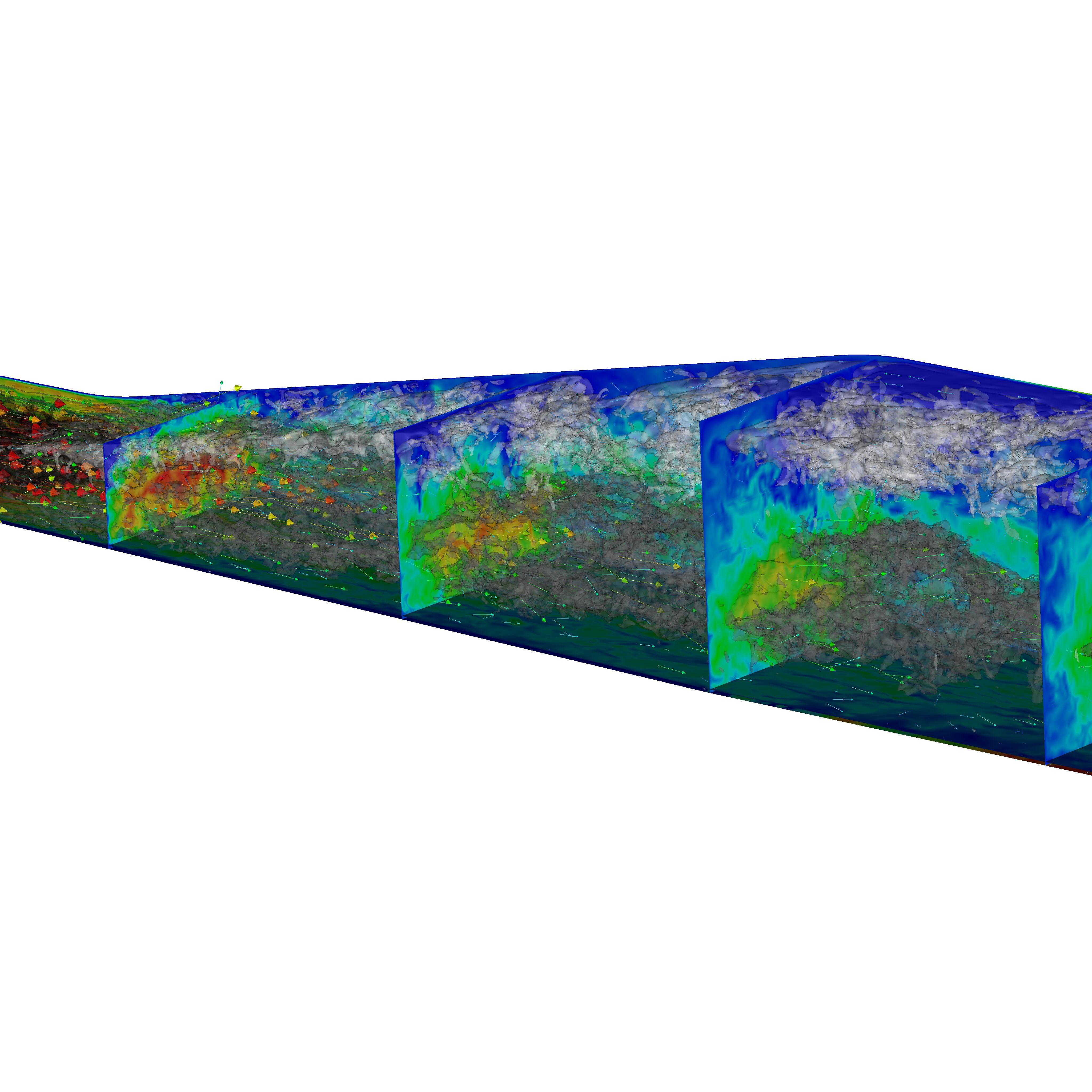
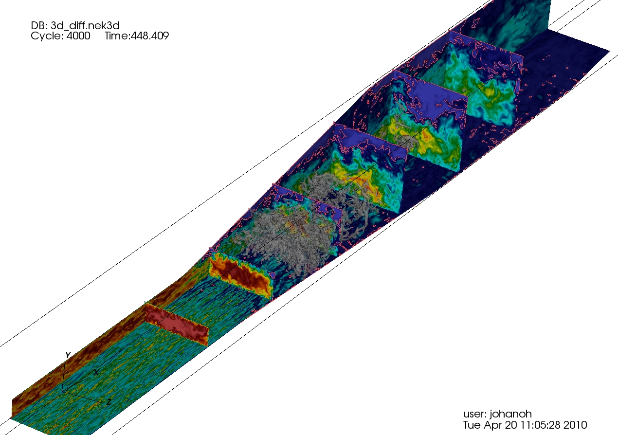
====Visualizations and computational mesh==== | |||
[[Media:UFR4-16_planes_press0000.jpeg|Crossflow planes with instantaneous streamwise velocity]] | |||
[[Media:UFR4-16_planes_nogrid_iso_vec.jpeg|Crossflow planes with instantaneous streamwise velocity and isosurfaces of streamwise velocity]] | |||
[[Media:UFR4-16_press_persp0010.jpeg|Instantaneous streamwise velocity in a spanwise midplane with some isosurfaces of instantaneous pressure]] | |||
[[Media:UFR4-16_mesh_paper.png|Mesh]] | |||
====Digitalized DNS database: full 3D mean velocity and Reynolds stress fields==== | |||
Explanation: | |||
*E.g., c13.2_Ucont2_KTH_DNS denotes the files comprising the contours of the axial velocity - Ucont - at the streamwise position ''x/h=2'' for the case 13.2 (ERCOFTAC SIG15 denotation). The same data are given at the streamwise locations ''x/h=2, 5, 8, 12'' and ''15'' | |||
*E.g., c13.2_urms2_KTH_DNS.txt denotes the file comprising the contours of the root-mean-square values of the streamwise stress component — urms — at the streamwise position ''x/h=2''. The same data are given at the streamwise locations ''x/h=2, 5, 8, 12'' and ''15'' | |||
*The file c13.2_cp_KTH_DNS.txt denotes the file comprising the pressure coefficient distribution at the bottom flat wall at the midpoint ''z/B=0.5'' | |||
*The file c13.2_z0250_x-2_KTH_DNS.txt denotes the file comprising all three mean velocity components, kinetic energy of turbulence and all six Reynolds stress components at the streamwise position ''x/h=-2'' (inflow duct) and the spanwise position ''z/B=0.25''. The same data are given at the streamwise locations ''x/h=0, 2, 4, 6, 8, 10, 12, 14, 15.5, 17, 18.5, 20'' and ''21.5'' at the following spanwise locations ''z/B=0.25, 0.5, 0.75'' and ''0.875''. | |||
{|align="center" border="1" cellpadding="5" | |||
|[[Media:c13.2_cp_KTH_DNS.txt|c13.2_cp_KTH_DNS.txt]] | |||
|- | |||
|[[Media:c13.2_Ucont2_KTH_DNS.txt|c13.2_Ucont2_KTH_DNS.txt]]||[[Media:c13.2_urms2_KTH_DNS.txt|c13.2_urms2_KTH_DNS.txt]] | |||
|- | |||
|[[Media:c13.2_Ucont5_KTH_DNS.txt|c13.2_Ucont5_KTH_DNS.txt]]||[[Media:c13.2_urms5_KTH_DNS.txt|c13.2_urms5_KTH_DNS.txt]] | |||
|- | |||
|[[Media:c13.2_Ucont8_KTH_DNS.txt|c13.2_Ucont8_KTH_DNS.txt]]||[[Media:c13.2_urms8_KTH_DNS.txt|c13.2_urms8_KTH_DNS.txt]] | |||
|- | |||
|[[Media:c13.2_Ucont12_KTH_DNS.txt|c13.2_Ucont12_KTH_DNS.txt]]||[[Media:c13.2_urms12_KTH_DNS.txt|c13.2_urms12_KTH_DNS.txt]] | |||
|- | |||
|[[Media:c13.2_Ucont15_KTH_DNS.txt|c13.2_Ucont15_KTH_DNS.txt]]||[[Media:c13.2_urms15_KTH_DNS.txt|c13.2_urms15_KTH_DNS.txt]] | |||
|- | |||
|[[Media:c13.2_z0250_x-2_KTH_DNS.txt|c13.2_z0250_x-2_KTH_DNS.txt]]||[[Media:c13.2_z0500_x-2_KTH_DNS.txt|c13.2_z0500_x-2_KTH_DNS.txt]] | |||
|[[Media:c13.2_z0750_x-2_KTH_DNS.txt|c13.2_z0750_x-2_KTH_DNS.txt]]||[[Media:c13.2_z0875_x-2_KTH_DNS.txt|c13.2_z0875_x-2_KTH_DNS.txt]] | |||
|- | |||
|[[Media:c13.2_z0250_x0_KTH_DNS.txt|c13.2_z0250_x0_KTH_DNS.txt]]||[[Media:c13.2_z0500_x0_KTH_DNS.txt|c13.2_z0500_x0_KTH_DNS.txt]] | |||
|[[Media:c13.2_z0750_x0_KTH_DNS.txt|c13.2_z0750_x0_KTH_DNS.txt]]||[[Media:c13.2_z0875_x0_KTH_DNS.txt|c13.2_z0875_x0_KTH_DNS.txt]] | |||
|- | |||
|[[Media:c13.2_z0250_x2_KTH_DNS.txt|c13.2_z0250_x2_KTH_DNS.txt]]||[[Media:c13.2_z0500_x2_KTH_DNS.txt|c13.2_z0500_x2_KTH_DNS.txt]] | |||
|[[Media:c13.2_z0750_x2_KTH_DNS.txt|c13.2_z0750_x2_KTH_DNS.txt]]||[[Media:c13.2_z0875_x2_KTH_DNS.txt|c13.2_z0875_x2_KTH_DNS.txt]] | |||
|- | |||
|[[Media:c13.2_z0250_x4_KTH_DNS.txt|c13.2_z0250_x4_KTH_DNS.txt]]||[[Media:c13.2_z0500_x4_KTH_DNS.txt|c13.2_z0500_x4_KTH_DNS.txt]] | |||
|[[Media:c13.2_z0750_x4_KTH_DNS.txt|c13.2_z0750_x4_KTH_DNS.txt]]||[[Media:c13.2_z0875_x4_KTH_DNS.txt|c13.2_z0875_x4_KTH_DNS.txt]] | |||
|- | |||
|[[Media:c13.2_z0250_x6_KTH_DNS.txt|c13.2_z0250_x6_KTH_DNS.txt]]||[[Media:c13.2_z0500_x6_KTH_DNS.txt|c13.2_z0500_x6_KTH_DNS.txt]] | |||
|[[Media:c13.2_z0750_x6_KTH_DNS.txt|c13.2_z0750_x6_KTH_DNS.txt]]||[[Media:c13.2_z0875_x6_KTH_DNS.txt|c13.2_z0875_x6_KTH_DNS.txt]] | |||
|- | |||
|[[Media:c13.2_z0250_x8_KTH_DNS.txt|c13.2_z0250_x8_KTH_DNS.txt]]||[[Media:c13.2_z0500_x8_KTH_DNS.txt|c13.2_z0500_x8_KTH_DNS.txt]] | |||
|[[Media:c13.2_z0750_x8_KTH_DNS.txt|c13.2_z0750_x8_KTH_DNS.txt]]||[[Media:c13.2_z0875_x8_KTH_DNS.txt|c13.2_z0875_x8_KTH_DNS.txt]] | |||
|- | |||
|[[Media:c13.2_z0250_x10_KTH_DNS.txt|c13.2_z0250_x10_KTH_DNS.txt]]||[[Media:c13.2_z0500_x10_KTH_DNS.txt|c13.2_z0500_x10_KTH_DNS.txt]] | |||
|[[Media:c13.2_z0750_x10_KTH_DNS.txt|c13.2_z0750_x10_KTH_DNS.txt]]||[[Media:c13.2_z0875_x10_KTH_DNS.txt|c13.2_z0875_x10_KTH_DNS.txt]] | |||
|- | |||
|[[Media:c13.2_z0250_x12_KTH_DNS.txt|c13.2_z0250_x12_KTH_DNS.txt]]||[[Media:c13.2_z0500_x12_KTH_DNS.txt|c13.2_z0500_x12_KTH_DNS.txt]] | |||
|[[Media:c13.2_z0750_x12_KTH_DNS.txt|c13.2_z0750_x12_KTH_DNS.txt]]||[[Media:c13.2_z0875_x12_KTH_DNS.txt|c13.2_z0875_x12_KTH_DNS.txt]] | |||
|- | |||
|[[Media:c13.2_z0250_x14_KTH_DNS.txt|c13.2_z0250_x14_KTH_DNS.txt]]||[[Media:c13.2_z0500_x14_KTH_DNS.txt|c13.2_z0500_x14_KTH_DNS.txt]] | |||
|[[Media:c13.2_z0750_x14_KTH_DNS.txt|c13.2_z0750_x14_KTH_DNS.txt]]||[[Media:c13.2_z0875_x14_KTH_DNS.txt|c13.2_z0875_x14_KTH_DNS.txt]] | |||
|- | |||
|[[Media:c13.2_z0250_x155_KTH_DNS.txt|c13.2_z0250_x155_KTH_DNS.txt]]||[[Media:c13.2_z0500_x155_KTH_DNS.txt|c13.2_z0500_x155_KTH_DNS.txt]] | |||
|[[Media:c13.2_z0750_x155_KTH_DNS.txt|c13.2_z0750_x155_KTH_DNS.txt]]||[[Media:c13.2_z0875_x155_KTH_DNS.txt|c13.2_z0875_x155_KTH_DNS.txt]] | |||
|- | |||
|[[Media:c13.2_z0250_x17_KTH_DNS.txt|c13.2_z0250_x17_KTH_DNS.txt]]||[[Media:c13.2_z0500_x17_KTH_DNS.txt|c13.2_z0500_x17_KTH_DNS.txt]] | |||
|[[Media:c13.2_z0750_x17_KTH_DNS.txt|c13.2_z0750_x17_KTH_DNS.txt]]||[[Media:c13.2_z0875_x17_KTH_DNS.txt|c13.2_z0875_x17_KTH_DNS.txt]] | |||
|- | |||
|[[Media:c13.2_z0250_x185_KTH_DNS.txt|c13.2_z0250_x185_KTH_DNS.txt]]||[[Media:c13.2_z0500_x185_KTH_DNS.txt|c13.2_z0500_x185_KTH_DNS.txt]] | |||
|[[Media:c13.2_z0750_x185_KTH_DNS.txt|c13.2_z0750_x185_KTH_DNS.txt]]||[[Media:c13.2_z0875_x185_KTH_DNS.txt|c13.2_z0875_x185_KTH_DNS.txt]] | |||
|- | |||
|[[Media:c13.2_z0250_x20_KTH_DNS.txt|c13.2_z0250_x20_KTH_DNS.txt]]||[[Media:c13.2_z0500_x20_KTH_DNS.txt|c13.2_z0500_x20_KTH_DNS.txt]] | |||
|[[Media:c13.2_z0750_x20_KTH_DNS.txt|c13.2_z0750_x20_KTH_DNS.txt]]||[[Media:c13.2_z0875_x20_KTH_DNS.txt|c13.2_z0875_x20_KTH_DNS.txt]] | |||
|- | |||
|[[Media:c13.2_z0250_x215_KTH_DNS.txt|c13.2_z0250_x215_KTH_DNS.txt]]||[[Media:c13.2_z0500_x215_KTH_DNS.txt|c13.2_z0500_x215_KTH_DNS.txt]] | |||
|[[Media:c13.2_z0750_x215_KTH_DNS.txt|c13.2_z0750_x215_KTH_DNS.txt]]||[[Media:c13.2_z0875_x215_KTH_DNS.txt|c13.2_z0875_x215_KTH_DNS.txt]] | |||
|} | |||
<br/> | |||
<br/> | |||
==Reference DNS and experimental data: mean flow and turbulence evolution== | |||
The following figures display and compare the reference experimental and | |||
DNS database results (the present results can be analysed along with the | |||
axial velocity contours shown in | |||
[[UFR_4-16_Test_Case#figure7|Figs. 7]] – | |||
[[UFR_4-16_Test_Case#figure9|9]] and [[UFR_4-16_Test_Case#figure13|13]]): | |||
In order to get an impression about the mean flow structure and about the | |||
available reference DNS and experimental results | |||
[[UFR_4-16_Test_Case#figure15|Figs. 15]] and | |||
[[UFR_4-16_Test_Case#figure16|16]] display | |||
the velocity field development in the vertical central plane of both | |||
diffusers (''z/B=0.5''; ''B=3.33 cm'' is the width of the inflow duct) typical for | |||
the flow in an expanding duct. The bulk flow exhibits deceleration, leading | |||
to an asymmetry of the velocity profile, particularly so for the axial | |||
velocity component. The effect of the adverse pressure gradient is | |||
especially visible in the flow region along the upper expanding wall. The | |||
velocity profile approaches gradually the form characterizing a separating | |||
flow, exhibiting regions of the zero velocity gradient (at separation and | |||
reattachment points) and profile inflection. The through-flow, that is the | |||
flow in the positive streamwise direction, is characterized by a spreading | |||
dictated by the pressure gradient arising from the geometry expansion. | |||
Accordingly, the position of the reduced velocity maximum is gradually | |||
shifted towards the upper wall, eventually reaching the center (''y/h=2'') of | |||
the straight outlet channel (with the height ''4h''). In this post-reattachment | |||
zone the velocity profile exhibits a fairly flattened form, being almost | |||
symmetric. The consequence of the velocity-profile flattening is a | |||
continuous monotonic decrease of the wall shear stress. The velocity | |||
profile evolution is similar in other longitudinal vertical planes. The | |||
specific differences are related to the vicinity of both bottom and upper | |||
walls, especially the latter upper wall, where the flow passes regions of | |||
three-dimensional flow reversal. | |||
<div id="figure15"></div> | |||
{|align="center" width="750" cellspacing="0" | |||
|style="border: 1px solid darkgray;"|[[Image:UFR4-16_figure15a.jpg|740px]] | |||
|- | |||
|style="border: 1px solid darkgray;"|[[Image:UFR4-16_figure15b.jpg|740px]] | |||
|- | |||
|style="border: 1px solid darkgray;"|[[Image:UFR4-16_figure15c.jpg|740px]] | |||
|- | |||
|'''Figure 15:''' Diffuser 1 - Evolution of the profiles of all three velocity components in the vertical plane ''x-y'' at the central spanwise locations ''z/B=1/2'' obtained experimentally and by means of DNS | |||
|} | |||
<div id="figure16"></div> | |||
{|align="center" width="750" cellspacing="0" | |||
|style="border: 1px solid darkgray;"|[[Image:UFR4-16_figure16a.jpg|740px]] | |||
|- | |||
|style="border: 1px solid darkgray;"|[[Image:UFR4-16_figure16b.jpg|740px]] | |||
|- | |||
|style="border: 1px solid darkgray;"|[[Image:UFR4-16_figure16c.jpg|740px]] | |||
|- | |||
|'''Figure 16:''' Diffuser 2 - Evolution of the profiles of all three velocity components in the vertical plane ''x-y'' at the central spanwise locations ''z/B=1/2'' obtained experimentally | |||
|} | |||
In the top part of [[UFR_4-16_Test_Case#figure17|Fig. 17 – upper]] | |||
the development of the streamwise | |||
turbulence intensity is shown for diffuser 1. The lowest turbulence | |||
intensity is situated in the region coinciding with the mean velocity | |||
maximum — flow zone with approximately zero velocity gradient — along the | |||
entire diffuser section. The Reynolds stress profiles exhibit their highest | |||
values in the regions with the most intensive flow deformation. These are | |||
the near-wall layer in the attached-flow regions and the flow zone along | |||
the shear layer bordering the recirculation zone. The peak of the | |||
turbulence intensity originating from the boundary layer at the top inflow | |||
duct wall increases initially, after the strong rise in pressure (see | |||
pressure coefficient development in | |||
[[UFR_4-16_Test_Case#figure11|Fig. 11]]), and weakens slightly after | |||
flow transition to the second part of the diffuser section, that is | |||
characterized by a decreasingly adverse pressure gradient. The streamwise | |||
turbulence intensity in the outlet duct is uniformly distributed over the | |||
cross-section. | |||
<div id="figure17"></div> | |||
{|align="center" width="750" cellspacing="0" | |||
|style="border: 1px solid darkgray;"|[[Image:UFR4-16_figure17a.jpg|740px]] | |||
|- | |||
|style="border: 1px solid darkgray;"|[[Image:UFR4-16_figure17b.jpg|740px]] | |||
|- | |||
|style="border: 1px solid darkgray;"|[[Image:UFR4-16_figure17c.jpg|740px]] | |||
|- | |||
|style="border: 1px solid darkgray;"|[[Image:UFR4-16_figure17d.jpg|740px]] | |||
|- | |||
|'''Figure 17:''' Diffuser 1 - Evolution of the profiles of the Reynolds stress components in the vertical plane ''x-y'' at the central spanwise locations ''z/B=1/2'' obtained experimentally and by means of DNS | |||
|} | |||
[[UFR_4-16_Test_Case#figure18|Fig. 18]] | |||
shows contour plots of the axial velocity component at five | |||
streamwise cross-sectional areas in both diffuser configurations obtained | |||
experimentally indicating the evolution of the flow separation pattern. The | |||
recirculation-zone development displayed here can be analyzed in parallel | |||
with the quantitative information about the fraction of the diffuser cross- | |||
sectional area occupied by the reverse flow depicted in | |||
[[UFR_4-16_Test_Case#figure19|Fig. 19]]. The | |||
adverse pressure gradient is imposed onto the intersecting boundary layers | |||
along flat walls upon entering the diffuser section. According to the | |||
experimental investigation the boundary layers along all walls are of | |||
comparable thickness. The separation starts immediately after the beginning | |||
of the diffuser section at ''x/L = 0 (x/h=0)''. The onset of separation is | |||
located in the upper-right diffuser corner, formed by the deflected side | |||
wall and the top wall, see e.g. the position ''x/h ≈ 2 (x/L=0.13)'' in | |||
[[UFR_4-16_Test_Case#figure19|Fig. 18]]. | |||
Initial growth of this corner bubble reveals its spreading rate along the | |||
two sloped walls being approximately of the same intensity, see position | |||
''x/h=5''. As the adverse pressure gradient along the upper wall outweighs | |||
significantly the one along the side wall due to the substantially higher | |||
angle of expansion in diffuser 1, 11.3° vs. 2.55°, the separation zone | |||
spreads gradually over the entire top wall surface, see position ''x/h=8''. The | |||
behaviour is different in diffuser 2. There one notes a strong three- | |||
dimensional nature of the separation pattern. The maximum occupation of the | |||
diffuser cross-sectional area by the flow reversal, around 22% and 15% for | |||
the diffusers 1 and 2, respectively | |||
([[UFR_4-16_Test_Case#figure19|Fig. 19]]), is documented at the | |||
position ''x/h=12-17 (x/L=0.8-1.13)''. The thickness of the flow reversal zone | |||
in the diffuser 1 (its dimension in the normal-to-wall direction) is almost | |||
constant over the diffuser width in this region, resembling approximately a | |||
2-D pattern. After this position the intensity of the back-flow weakens. | |||
The experimental results indicate that the reattachment region is located | |||
within the straight outlet duct, | |||
[[UFR_4-16_Test_Case#figure19|Fig. 19]]. The separation pattern and the | |||
differences between diffuser 1 and 2 can also be seen clearly from the 3D | |||
plots given in | |||
[[UFR_4-16_Evaluation#figure26|Fig. 26]], which were obtained by LES. | |||
<div id="figure18"></div> | |||
{|align="center" width="750" cellspacing="0" | |||
|colspan="2" style="border: 1px solid darkgray;"|[[Image:UFR4-16_figure18.png|740px]] | |||
|- | |||
|style="border: 1px solid darkgray;" align="center"|'''Diffuser 1''' | |||
|style="border: 1px solid darkgray;" align="center"|'''Diffuser 2''' | |||
|- | |||
|colspan="2"|'''Figure 18:''' Comparison between experimentally obtained iso-contours of the axial velocity field in the cross planes ''y-z'' at five selected streamwise locations within the both diffuser section (the thick line denotes the zero-velocity line). From [[UFR_4-16_References#7|Cherry ''et al.'' (2008)]] | |||
|} | |||
<div id="figure19"></div> | |||
{|align="center" width="750" | |||
|[[Image:UFR4-16_figure19.png|740px]] | |||
|- | |||
|'''Figure 19:''' Fraction of the cross-sectional area occupied by the flow reversal in both diffuser configurations. From [[UFR_4-16_References#7|Cherry ''et al.'' (2008)]] | |||
|} | |||
<br/> | <br/> | ||
---- | ---- | ||
Latest revision as of 10:57, 13 December 2021
Flow in a 3D diffuser
Confined flows
Underlying Flow Regime 4-16
Test Case Study
Brief description of the test case studied
The diffuser shapes, dimensions and the coordinate system are shown in Fig. 3 and Fig. 4. Both diffuser configurations considered have the same fully‐developed flow at channel inlet but slightly different expansion geometries: the upper-wall expansion angle is reduced from 11.3° (Diffuser 1) to 9° (Diffuser 2) and the side-wall expansion angle is increased from 2.56° (Diffuser 1) to 4° (Diffuser2). The flow in the inlet duct (height h=1 cm, width B=3.33 cm) corresponds to fully-developed turbulent channel flow (enabled experimentally by a development channel being 62.9 channel heights long). The L=15h long diffuser section is followed by a straight outlet part (12.5h long). Downstream of this the flow goes through a 10h long contraction into a 1 inch diameter tube. The curvature radius at the walls transitioning between diffuser and the straight duct parts are 6 cm (Diffuser 1) and 2.8 cm (Diffuser 2). The bulk velocity in the inflow duct is in the x-direction resulting in the Reynolds number based on the inlet channel height of 10000. The origin of the coordinates (y=0, z=0) coincides with the intersection of the two non-expanding walls at the beginning of the diffuser's expansion (x=0). The working fluid is water (ρ=1000 kg/m3 and μ=0.001 Pas).


|
| Figure 3: Geometry of the 3-D diffuser 1 considered (not to scale), Cherry et al. (2008); see also Jakirlić et al. (2010a) |

|
| Figure 4: Geometry of the 3-D diffuser 2 considered (not to scale), Cherry et al. (2008). |
Experimental investigation
Brief description of the experimental setup
The measurements were performed in a recirculating water channel using the method of magnetic resonance velocimetry (MRV), Fig. 5. MRV makes use of a technique very similar to that used in conventional medical magnetic resonance imaging (MRI), Fig. 6. Experiments were performed on a 1.5 Tesla magnet with resolution of 0.9 x 0.9 x 0.9 mm and a 7 Tesla magnet with resolution of 0.4 x 0.4 x 0.4 mm. Interested readers are referred to Cherry et al. (2008, 2009) for more details about the measurement technique.

|

|
| Figure 5: Schematic of the experimental flow system (upper) and design of the 3D diffuser. Courtesy of J. Eaton (Stanford University) |

|
| Figure 6: 3D diffuser arrangement in a medical magnetic resonance imaging device. Courtesy of J. Eaton (Stanford University) |
Mean velocity and Reynolds stress measurements
Cherry et al. provided a detailed reference database comprising the three-component mean velocity field and the streamwise Reynolds stress component field within the entire diffuser section. Both diffuser configurations considered are characterized by a three-dimensional boundary-layer separation, but the slightly different expansion geometries caused the size and shape of the separation bubble exhibiting a high degree of geometric sensitivity to the dimensions of the diffuser as illustrated in Figs. 7, 8 and 9

|
| Figure 7: Streamwise velocity contours in a plane parallel to the top wall, from Cherry et al. (2008) |

| ||

| ||
 |
 |

|
| Figure 8: Measured streamwise velocity contours in the central plane (upper) of the Diffuser 1 and in the three selected cross-sectional slices positioned at different distances from the diffuser inlet (lower; their locations are denoted by thick white lines in the upper figure). Note that the black line indicates zero streamwise velocity and the purple and pink regions are reverse flow. The velocity values are normalized by the bulk inlet velocity being Vref=1 m/s. Courtesy of J. Eaton (Stanford University) | ||

| ||

|

|

|
| Figure 9: Measured streamwise velocity contours in the central plane (upper) of the Diffuser 2 and in the three selected cross-sectional slices positioned at different distances from the diffuser inlet (lower; their locations are denoted by thick white lines in the upper figure). Note that the black line indicates zero streamwise velocity and the purple and pink regions are reverse flow. The velocity values are normalized by the bulk inlet velocity being Vref=1 m/s. Courtesy of J. Eaton (Stanford University) | ||
| x/h=2 | x/h=5 | x/h=8 | x/h=12 | x/h=15 |
|---|---|---|---|---|

|

|

|

|

|
| Figure 10: Measurements of turbulent streamwise stress components taken in cross-sectional slices of the diffuser 1 perpendicular to the mean flow. The region of highest turbulence (red areas; ignore the red areas at the bottom walls) follows the shear layer between forward and reverse flow. h=1cm represents the height of the inflow duct. Courtesy of J. Eaton (Stanford University) | ||||
Pressure measurements
In addition Cherry et al. (2009) provided the pressure distribution along the bottom non-deflected wall of diffuser 1 at different Reynolds numbers. Complementary to the Reynolds number 10000 (for which the entire flow field was measured), two higher Reynolds numbers — 20000 and 30000 — were also considered, Fig. 11. The surface pressure distribution was evaluated to yield the coefficient ; the reference pressure was taken at the position x/L = 0.05. The pressure curve exhibits a development typical of flow in diverging ducts. The pressure decrease in the inflow duct is followed by a steep pressure increase already at the very end of the inflow duct and especially at the beginning of the diffuser section. The transition from the initial strong pressure rise to its moderate increase occurs at x/L ≈ 0.3, (x/h=4.5) corresponding to the position where about 5% of the entire cross-section is occupied by the flow reversal (see e.g., Fig. 19. The onset of separation causes a certain contraction of the flow cross‐section, leading to a weakening of the deceleration intensity and, accordingly, to a slower pressure increase. The region characterized by a monotonic pressure rise was reached in the remainder of the diffuser section.


|
| Figure 11: Pressure recovery coefficients relative to the pressure on the bottom wall of the diffuser 1 inlet in a range of flow Reynolds number. L=15 cm represents the length of Diffuser 1, from Cherry et al. (2009) |
Measurements uncertainties
(adopted from Cherry et al., 2008, IJHFF, Vol. 29(3))
Elkins et al. (2004) estimated the maximum relative uncertainty of individual mean velocity measurements to be about 10% of the measured value in a similar highly turbulent flow. However, comparisons to PIV in a backward facing step flow (Elkins et al., 2007) show that only a small percentage of MRV velocity samples deviate by that much and most are much more accurate. To test this, the streamwise velocity component was integrated over 250 cross-sections of the MRV data and the results were compared to the known volume flow rate. This indicated an uncertainty in the integral of less than 2% with a 95% confidence level.
Measurements of turbulent normal stresses in Diffuser 1 were also taken using the MR technique described by Elkins et al. (2007). This method is based on diffusion imaging principles in which the turbulence causes a loss of net magnetization signal from a voxel in the flow. This causes a decay in signal strength which can be related to turbulent velocity statistics. Elkins et al found this method to be accurate within 20% everywhere in the FOV and within 5% in regions of high turbulence. Three turbulence scans were completed using three different magnetic field gradient strengths. For each gradient strength, 30 scans were completed and averaged. The three averaged data sets were then averaged to obtain a final data set.
Experimental data available
Velocity, (and streamwise Reynolds stress components for diffuser 1) and coordinate data for both diffusers are available here.
| Diffuser 1 data.zip (contains 1 file, 8.4 MBytes) |
| Diffuser 1 turbulence.zip (contains 1 file, 5.3 MBytes) |
| Diffuser 2 data.zip (contains 1 file, 4 MBytes) |
The data are seven 3D matlab matrices. The x, y, and z matrices give the coordinates of each point in the coordinate system shown in Fig. 5. The units are meters. The Vx, Vy, and Vz matrices give the corresponding velocity components for each point in m/sec. The matrix mg gives the relative signal magnitude detected by the MRI machine.
Experimental data for the pressure coefficient in Diffuser 1 for the inflow Reynolds number Re=10000 are available here (Cp_Re=10000.xlsx). The coordinate system is the same as the coordinate system described in the corresponding manuscript (see below). is defined as , where is the pressure at x=0.05 (see Fig. 11) at the midpoint (z/B=0.5) of the bottom flat wall (opposite the wall expanding at 11.3 degrees), is the density, and is the bulk inlet velocity. The data were taken in a line along the bottom wall of Diffuser 1 at constant y and z coordinates. L (=15 cm) indicates the length of the diffuser.


Please acknowledge the authors of the experiment when using their database!
CFD Methods
The flow in the present diffuser configuration was intensively investigated computationally in the framework of two ERCOFTAC-SIG15 Workshops and in the European ATAAC project. The workshops focussing on both 3D diffuser configurations (denoted by SIG15 Case 13.2-1 and SIG15 Case 13.2-2, respectively) were organized at the Technical University of Graz, Austria in September, 2008 and the "LA Sapienza" University of Rome, Italy in September, 2009. The corresponding reports are published in the ERCOFTAC Bulletin Issues, Steiner et al. (2009) and Jakirlić et al. (2010b), see "List of References". Both in the workshops and in the ATAAC project a wide range of turbulence models in both LES and RANS frameworks as well as some novel Hybrid LES/RANS formulations have been employed. The computational database was furthermore enriched by the results of a Direct Numerical Simulation of the first diffuser performed by Ohlsson et al. (2010). The list of all computational contributions to the workshops including some basic information about the methods and models used and corresponding grid resolution is given in the following tables 1 and table 2. For more computational details, interested readers are referred to the "workshop proceedings" — see the corresponding links at the end of the Section "Evaluation of the results". The results from the ATAAC project and information on the methods used can be obtained through the links ATAAC_D3-2-36_excerpt3DDiffuser.pdf (excerpt from an ATAAC report) and [ATAAC_finalWorkshop_ST04-Diffuser-ANSYS.pdf] (PowerPoint presentation at ATAAC final workshop).

|
| Table 1: SIG15 Case 13.2-1 (Diffuser 1) — contributors and methods (note that the DNS grid comprises 220 million cells in the follow-up work published in Ohlsson et al. (2010)) |
| N.B. ITS is "Institut für Thermische Strömungsmaschinen" |

|
| Table 2: SIG15 Case 13.2-2 (Diffuser 2) — contributors and methods |
| N.B. ITS is "Institut für Thermische Strömungsmaschinen" |
Direct numerical simulation of the flow in a 3D diffuser
(adopted from Ohlsson et al., 2010, JFM, Vol. 650)
In this part of the present contribution the DNS study of the flow in 3D Diffuser 1 performed recently by Ohlsson et al. (2010) will be described in more details. Ohlsson et al. participated with this contribution at the 14th SIG15 Workshop on Refined Turbulence Modeling (Jakirlić et al., 2010b). Accordingly, their results are also part of the CFD methods/models evaluation — along with the results obtained by different LES, RANS and Hybrid LES/RANS models (see the next chapter). In addition, as the DNS provided a very comprehensive database comprising all three mean velocity components (and associated integral characteristics such as surface pressure and friction factor) and all six Reynolds stress components as well as a certain insight into the physics (not detected by the experimental investigation) one can regard it also as a reference investigation, as we do presently.
The Direct Numerical Simulation of the Diffuser 1 was performed using a massively parallel high-order spectral element code. The incompressible Navier-Stokes equations are solved using a Legendre-polynomial-based spectral-element method, implemented in the code nek5000, developed by Fischer et al. (2008). The computational domain shown in Fig. 12 is set up in close agreement with the diffuser geometry in the experiment (see Fig.3) and consists of the inflow development duct of almost 63 duct heights, h, (starting at the non-dimensional coordinate x = -62.9), the diffuser expansion located at x = 0 and the converging section upstream of the outlet. The corners resulting from the diffuser expansion are smoothly rounded with a radius of 6.0 in accordance with the experimental set-up. The maximum dimensions are Lx =105.4 h, Ly =[h, 4h], Lz =[3.33 h, 4h]. In the inflow duct, laminar flow undergoes natural transition by the use of an unsteady trip forcing (see e.g. Schlatter et al., 2009), which avoids the use of artificial turbulence and eliminates artificial temporal frequencies which may arise from inflow recycling methods (Herbst et al., 2007). A 'sponge region' is added at the end of the contraction in order to smoothly damp out turbulent fluctuations, thereby eliminating spurious pressure waves. It is followed by a homogeneous Dirichlet condition for the pressure and a homogeneous Neumann condition for the velocities. The resolution of approximately 220 million grid points is obtained by a total of 127750 local tensor product domains (elements) with a polynomial order of 11, respectively, resulting in Δz+max≈11.6, Δy+max≈13.2 and Δx+max≈19.5 in the duct center and the first grid point being located at z+≈0.074 and y+≈0.37, respectively (note that at the time of the ERCOFTAC SIG15 workshop the DNS grid had 172 million grid points, see Chapter "Evaluation"). It was verified that this resolution yields accurate results in turbulent channel flow simulations. In the diffuser, the grid is linearly stretched in both directions, but since the mean resolution requirements decreases with the velocity, which decreases linearly with the area expansion, the resolution in the entire domain is hence satisfactory. The simulation was performed on the Blue Gene/P at ALCF, Argonne National Laboratory (32768 cores and a total of 8 million core hours) and on the cluster 'Ekman' at PDC, Stockholm (2048 cores and a total of 4 million core hours). Thirteen flow-through times, t Ub/L=13, based on bulk velocity, Ub, and diffuser length, L=15 h, were simulated in order to let the flow settle to an equilibrium state before turbulent statistics were collected over approximately Ubt/L=21 additional flow-through times.
In addition to the three-dimensional mean velocity field, all six Reynolds stress components were evaluated, as well as the surface pressure and skin friction distribution along the bottom wall.

|
| Figure 12: DNS grid of the diffuser 1 geometry showing the development region, diffuser expansion, converging section and outlet. From Ohlsson et al. (2010) |
Fig. 13 illustrates the mean axial flow field obtained by DNS along with
the experimental data and Fig. 14 depicts the skin friction evolution along
the bottom diffuser wall at the midpoint
(z/B=0.5; Cf=τwall / (0.5ρU2bulk) ). The latter DNS
result was evaluated exclusively for the needs of the 14th ERCOFTAC
Workshop; it is not part of the DNS database which can be downloaded here.

| |||||||||||||||||||||||||||||
| Figure 13: Cross-flow planes of streamwise velocity component at 2, 5, 8 and 15 h downstream of the diffuser throat. Left: DNS. Right: Experiment by Cherry et al. (2008). Each streamwise position has its own colour bar on the right. Contour lines are spaced 0.1 Vref apart. Thick black lines correspond to the zero velocity contour. From Ohlsson et al. (2010)
|
|||||||||||||||||||||||||||||


