AC 6-10 Evaluation: Difference between revisions
David.Fowler (talk | contribs) |
m (Dave.Ellacott moved page Silver:AC 6-10 Evaluation to AC 6-10 Evaluation over redirect) |
||
| (10 intermediate revisions by 3 users not shown) | |||
| Line 1: | Line 1: | ||
{{AC|front=AC 6-10|description=AC 6-10 Description|testdata=AC 6-10 Test Data|cfdsimulations=AC 6-10 CFD Simulations|evaluation=AC 6-10 Evaluation|qualityreview=AC 6-10 Quality Review|bestpractice=AC 6-10 Best Practice Advice| | {{AC|front=AC 6-10|description=AC 6-10 Description|testdata=AC 6-10 Test Data|cfdsimulations=AC 6-10 CFD Simulations|evaluation=AC 6-10 Evaluation|qualityreview=AC 6-10 Quality Review|bestpractice=AC 6-10 Best Practice Advice|relatedUFRs=AC 6-10 Related ACs}} | ||
| Line 578: | Line 578: | ||
== Wake Profiles == | == Wake Profiles == | ||
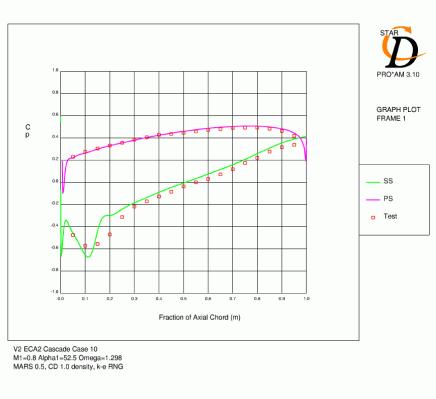
Wake profiles for case 3 at the exit traverse plane for the three meshes are shown in [ | Wake profiles for case 3 at the exit traverse plane for the three meshes are shown in [[AC 6-10 Evaluation#Figure4.1|Figure 4.1]]. The results are plotted from mid-passage to mid-passage (i.e. over the pitchwise extent of the computational domain) from pressure side to suction side. As there is no information confirming the datum position of the experimental results the accuracy of the wake alignment is uncertain. The wake depth is generally over-predicted, although the width is less than experiment at the base of the profile for mesh A. Mesh C gives the best result in terms of wake size and shape. | ||
The results on mesh C for the six operating points are shown in [ | The results on mesh C for the six operating points are shown in [[AC 6-10 Evaluation#Figure4.2|Figure 4.2]]. Again, wake depth is usually slightly high, but generally agreement with experiment is good. Case 9 (for which under-prediction of overall loss was particularly large) shows a much reduced predicted loss coefficient on the suction side. However, the experimental results do show pitchwise non-periodicity, possibly indicating additional loss from 3D flow features. | ||
== Surface pressure distributions == | == Surface pressure distributions == | ||
The predictions of surface pressure distribution for case 3 ([ | The predictions of surface pressure distribution for case 3 ([[AC 6-10 Evaluation#Figure4.3|Figure 4.3]]) were reasonably accurate for all meshes. The initial deceleration after the suction surface peak was too rapid, which lead to high pressure over the remainder of the blade for meshes A and B. As the minimum pressure on the suction side was slightly low for mesh C, the distribution over the rear of the blade is actually closer. The location of minimum pressure on the suction surface is most accurate for mesh C. At the trailing edge, STAR predicts a small region of negative loading which is due to the acceleration of the pressure side flow around the trailing edge and the separated boundary layer on the suction side. The O-grid topology of mesh C reduces the size of this region to a minimum (see section 4.4). | ||
[[AC 6-10 Evaluation#Figure4.4|Figures 4.4]], [[AC 6-10 Evaluation#Figure4.5|4.5]], [[AC 6-10 Evaluation#Figure4.6|4.6]], [[AC 6-10 Evaluation#Figure4.7|4.7]], [[AC 6-10 Evaluation#Figure4.8|4.8]] and [ | [[AC 6-10 Evaluation#Figure4.4|Figures 4.4]], [[AC 6-10 Evaluation#Figure4.5|4.5]], [[AC 6-10 Evaluation#Figure4.6|4.6]], [[AC 6-10 Evaluation#Figure4.7|4.7]], [[AC 6-10 Evaluation#Figure4.8|4.8]] and [[AC 6-10 Evaluation#Figure4.9|4.9]] show contours of Mach number and distribution of pressure coefficient over the blade for all six cases with mesh C. The agreement for the Cp distributions is generally quite good. For cases 1 and 2, which have lower inlet mach numbers, the acceleration over the leading edge region is slightly under-predicted and the subsequent pressure over the rest of the suction surface is high as a result. For the remaining cases with a 0.8 inlet Mach number, the minimum pressure tends to be low and the subsequent diffusion following this peak over-predicted. The location of the suction surface peak and the pressure coefficient at the trailing edge are generally very accurate. | ||
The results for case 9 ([[AC 6-10 Evaluation#Figure4.8|Figure 4.8]]) show similar features to those described above, but the accuracy compared to the experiment is less good. The leading edge loading is increased due to the higher inlet angle (as in case 10) which can be seen in the Mach number contours and the rate of diffusion is significantly higher than the experimental data. The predicted pressure level at the trailing edge is high. | The results for case 9 ([[AC 6-10 Evaluation#Figure4.8|Figure 4.8]]) show similar features to those described above, but the accuracy compared to the experiment is less good. The leading edge loading is increased due to the higher inlet angle (as in case 10) which can be seen in the Mach number contours and the rate of diffusion is significantly higher than the experimental data. The predicted pressure level at the trailing edge is high. | ||
| Line 594: | Line 594: | ||
The boundary layer development from the leading edge is of crucial importance when making accurate predictions of this type of geometry. Improvements over the sheared H grids have been made by changing to an O-type topology to ensure a completely smooth leading edge shape and to improve the orthogonality of the mesh. The recently developed 'ESTurbo' automatic grid generator for turbomachinery geometries provided by the CD-adapco Group has been used to generate such a mesh. But in fact the most significant improvements provided by mesh C appear to be at the trailing edge. | The boundary layer development from the leading edge is of crucial importance when making accurate predictions of this type of geometry. Improvements over the sheared H grids have been made by changing to an O-type topology to ensure a completely smooth leading edge shape and to improve the orthogonality of the mesh. The recently developed 'ESTurbo' automatic grid generator for turbomachinery geometries provided by the CD-adapco Group has been used to generate such a mesh. But in fact the most significant improvements provided by mesh C appear to be at the trailing edge. | ||
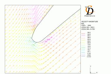
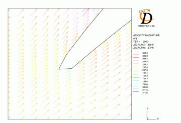
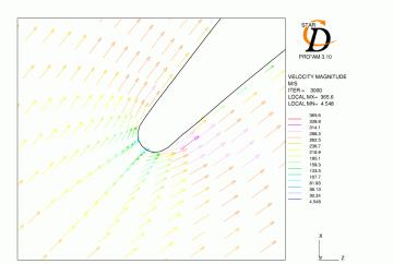
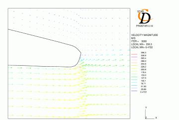
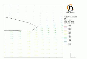
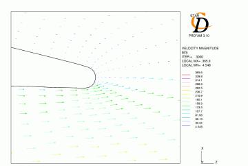
[ | [[AC 6-10 Evaluation#Figure4.10|Figure 4.10]] and [[AC 6-10 Evaluation#Figure4.11|4.11]] show detailed views of flow vectors at the leading and trailing edges for case 3. The trailing edge vectors for mesh A show that the pressure surface flow does not leave the blade at a tangent to the pressure surface, but rather accelerates round the trailing edge circle and hence affects deviation. For mesh C this effect is significantly reduced. The improvements from mesh C are connected with the higher quality cells in this region as well as a better definition of blade shape. In the extreme case of mesh B it can be seen that the trailing edge shape heavily influences the exit flow angle. The effect of different turbulence models on this aspect of the flow could be also be investigated. A higher density O-mesh should also be used to investigate grid independence. | ||
In reality there will be an initial laminar region from the leading edge, with the length of the region and the subsequent transition dependent on the inlet conditions. The use of wall functions in the present model means this boundary layer development cannot be predicted. Improved understanding could be gained by comparison of velocity profiles through the boundary layer with experimental data. | In reality there will be an initial laminar region from the leading edge, with the length of the region and the subsequent transition dependent on the inlet conditions. The use of wall functions in the present model means this boundary layer development cannot be predicted. Improved understanding could be gained by comparison of velocity profiles through the boundary layer with experimental data. | ||
| Line 604: | Line 604: | ||
An O-mesh topology around the blade and an H-grid upstream and downstream gives good definition of the blade geometry. In addition, economic clustering of cells in regions of high gradient can be easily achieved. This gave good predictions of deviation and loss at design incidence, although loss was generally slightly low. Deviation in particular improved with the O mesh. Wake profiles were generally slightly deep, with wake width in better agreement. Surface pressure distributions were accurately predicted with locations of suction surface peaks improving with the O mesh. | An O-mesh topology around the blade and an H-grid upstream and downstream gives good definition of the blade geometry. In addition, economic clustering of cells in regions of high gradient can be easily achieved. This gave good predictions of deviation and loss at design incidence, although loss was generally slightly low. Deviation in particular improved with the O mesh. Wake profiles were generally slightly deep, with wake width in better agreement. Surface pressure distributions were accurately predicted with locations of suction surface peaks improving with the O mesh. | ||
Boundary layer growth over the blade is a very important aspect of modelling this type of flow. A good definition of the leading edge will help to give the correct flow acceleration and boundary layer thickness as the flow develops. The trailing edge shape can have a strong influence on exit flow angle, especially when unrefined. The O mesh improved this aspect of the model significantly. Higher densities of O-mesh should also be investigated. Improved understanding could be gained by comparison of boundary layer parameters. The use of wall functions with the k- | Boundary layer growth over the blade is a very important aspect of modelling this type of flow. A good definition of the leading edge will help to give the correct flow acceleration and boundary layer thickness as the flow develops. The trailing edge shape can have a strong influence on exit flow angle, especially when unrefined. The O mesh improved this aspect of the model significantly. Higher densities of O-mesh should also be investigated. Improved understanding could be gained by comparison of boundary layer parameters. The use of wall functions with the k-ε turbulence model will become less accurate as the velocity profile differs from the law of the wall, for example during laminar-turbulent transition at the leading edge and in the adverse pressure gradient over the rear of the blade. Further investigations could look at low-Re or two-layer models. | ||
Further work is planned to model the remaining test conditions for which there is experimental data, and to utilise more of the models available within STAR-CD.<br style="page-break-before: always" clear="all" /> | Further work is planned to model the remaining test conditions for which there is experimental data, and to utilise more of the models available within STAR-CD.<br style="page-break-before: always" clear="all" /> | ||
<span id="Figure4.1"></span> | |||
<center>[[Image:A6-10d30_files_image045.gif]]</center> | <center>[[Image:A6-10d30_files_image045.gif]]</center> | ||
| Line 622: | Line 623: | ||
<center>Figure 4.1 Comparison of wake profiles for different meshes (Case 3)<br style="page-break-before: always" clear="all" /></center> | <center>Figure 4.1 Comparison of wake profiles for different meshes (Case 3)<br style="page-break-before: always" clear="all" /></center> | ||
<span id="Figure4.2"></span> | |||
{| align="left" | {| align="left" | ||
| width="59" height="2" | | | width="59" height="2" | | ||
| Line 681: | Line 683: | ||
<center> </center> | <center> </center> | ||
<span id="Figure4.3"></span> | |||
<center>[[Image:A6-10d30_files_image057.jpg]]</center> | <center>[[Image:A6-10d30_files_image057.jpg]]</center> | ||
| Line 696: | Line 698: | ||
<center>Figure 4.3 Comparison of surface pressure distributions for different meshes (Case 3)</center> | <center>Figure 4.3 Comparison of surface pressure distributions for different meshes (Case 3)</center> | ||
<span id="Figure4.4"></span> | |||
<center>[[Image:A6-10d30_files_image063.jpg]]</center> | <center>[[Image:A6-10d30_files_image063.jpg]]</center> | ||
| Line 702: | Line 705: | ||
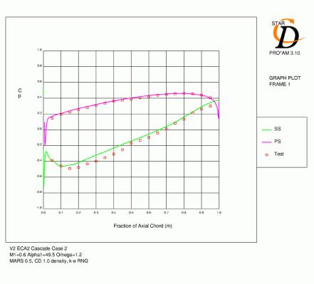
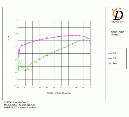
<center>Figure 4.4 Mach number contours and surface pressure distribution. Case 1. (Mesh C)<br style="page-break-before: always" clear="all" /></center> | <center>Figure 4.4 Mach number contours and surface pressure distribution. Case 1. (Mesh C)<br style="page-break-before: always" clear="all" /></center> | ||
<span id="Figure4.5"></span> | |||
<center>[[Image:A6-10d30_files_image067.jpg]]</center> | <center>[[Image:A6-10d30_files_image067.jpg]]</center> | ||
| Line 710: | Line 714: | ||
<center>Figure 4.5 Mach number contours and surface pressure distribution. Case 2. (Mesh C)<br style="page-break-before: always" clear="all" /> </center> | <center>Figure 4.5 Mach number contours and surface pressure distribution. Case 2. (Mesh C)<br style="page-break-before: always" clear="all" /> </center> | ||
<span id="Figure4.6"></span> | |||
<center>[[Image:A6-10d30_files_image071.jpg]]</center> | <center>[[Image:A6-10d30_files_image071.jpg]]</center> | ||
| Line 716: | Line 721: | ||
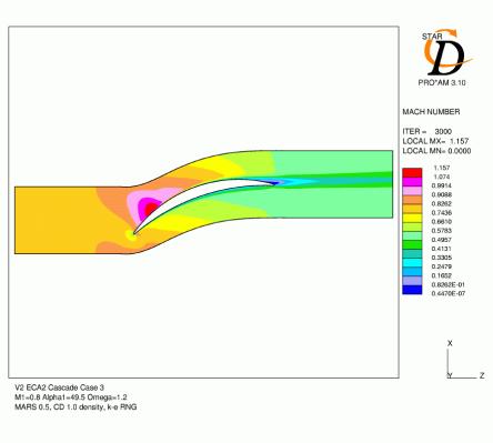
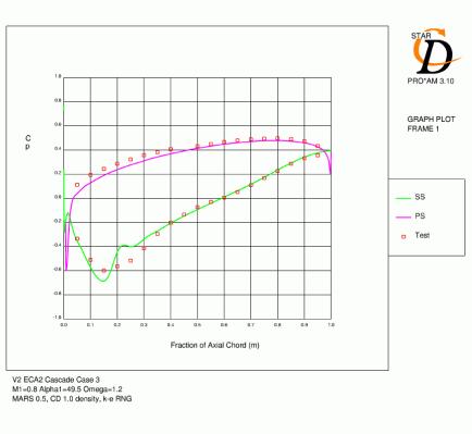
<center>Figure 4.6 Mach number contours and surface pressure distribution. Case 3. (Mesh C)<br style="page-break-before: always" clear="all" /> </center> | <center>Figure 4.6 Mach number contours and surface pressure distribution. Case 3. (Mesh C)<br style="page-break-before: always" clear="all" /> </center> | ||
<span id="Figure4.7"></span> | |||
<center>[[Image:A6-10d30_files_image074.jpg]]</center> | <center>[[Image:A6-10d30_files_image074.jpg]]</center> | ||
| Line 724: | Line 730: | ||
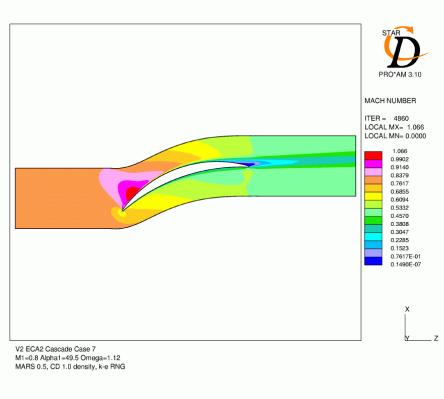
<center>Figure 4.7 Mach number contours and surface pressure distribution. Case 7. (Mesh C)<br style="page-break-before: always" clear="all" />[[Image:A6-10d30_files_image078.jpg]]</center> | <center>Figure 4.7 Mach number contours and surface pressure distribution. Case 7. (Mesh C)<br style="page-break-before: always" clear="all" />[[Image:A6-10d30_files_image078.jpg]]</center> | ||
<span id="Figure4.8"></span> | |||
<center>[[Image:A6-10d30_files_image080.jpg]]</center> | <center>[[Image:A6-10d30_files_image080.jpg]]</center> | ||
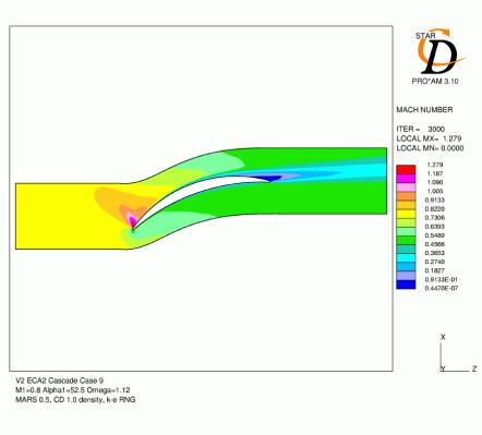
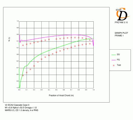
<center>Figure 4.8 Mach number contours and surface pressure distribution. Case 9. (Mesh C)<br style="page-break-before: always" clear="all" /> </center> | <center>Figure 4.8 Mach number contours and surface pressure distribution. Case 9. (Mesh C)<br style="page-break-before: always" clear="all" /> </center> | ||
<span id="Figure4.9"></span> | |||
<center>[[Image:A6-10d30_files_image082.jpg]]</center> | <center>[[Image:A6-10d30_files_image082.jpg]]</center> | ||
| Line 734: | Line 742: | ||
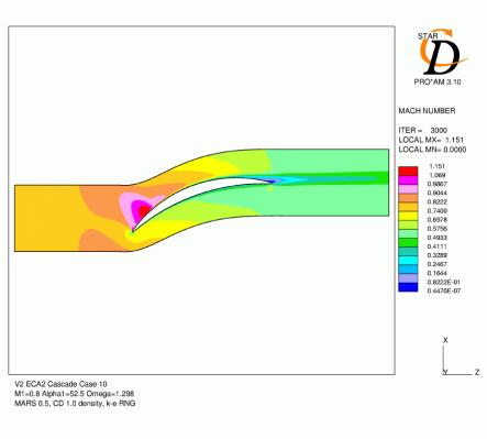
<center>Figure 4.9 Mach number contours and surface pressure distribution. Case 10. (Mesh C)</center> | <center>Figure 4.9 Mach number contours and surface pressure distribution. Case 10. (Mesh C)</center> | ||
<span id="Figure4.10"></span> | |||
<center>[[Image:A6-10d30_files_image086.jpg]]</center> | <center>[[Image:A6-10d30_files_image086.jpg]]</center> | ||
| Line 748: | Line 757: | ||
<center>Figure 4.10 Velocity vectors at the leading edge. Case 3.</center> | <center>Figure 4.10 Velocity vectors at the leading edge. Case 3.</center> | ||
<span id="Figure4.11"></span> | |||
<center>[[Image:A6-10d30_files_image092.jpg]]</center> | <center>[[Image:A6-10d30_files_image092.jpg]]</center> | ||
| Line 769: | Line 779: | ||
{{AC|front=AC 6-10|description=AC 6-10 Description|testdata=AC 6-10 Test Data|cfdsimulations=AC 6-10 CFD Simulations|evaluation=AC 6-10 Evaluation|qualityreview=AC 6-10 Quality Review|bestpractice=AC 6-10 Best Practice Advice| | {{AC|front=AC 6-10|description=AC 6-10 Description|testdata=AC 6-10 Test Data|cfdsimulations=AC 6-10 CFD Simulations|evaluation=AC 6-10 Evaluation|qualityreview=AC 6-10 Quality Review|bestpractice=AC 6-10 Best Practice Advice|relatedUFRs=AC 6-10 Related ACs}} | ||
Latest revision as of 18:42, 11 February 2017
Axial compressor cascade
Application Challenge 6-10 © copyright ERCOFTAC 2004
Evaluation
Overall performance
Tables 4.1 to 4.5 summarise the experimental data and STAR predictions, respectively, for a range of operating conditions. Exit Mach number was in reasonable agreement with the experimental data, typically within about 2%. Mesh A over-predicts the exit flow angle significantly by between 2-5°. Mesh B also over-predicts for case 3. This would indicate more deviation and hence earlier and larger flow separation from the suction surface but the behaviour of the flow on the pressure surface as it leaves the trailing edge is probably the main factor (see section 4.4). The results for mesh C are much closer to experiment and for cases with the design inlet angle of 49.5°, exit flow angle is within 0.5°. For the higher inlet flow angle the disagreement is larger, up to 2°. However the largest discrepancy is for case 9, for which there is some doubt over the experimental data (see below). Overall pressure loss is low for both meshes, although closer to experiment for mesh C.
|
|
|
|
|
|
|
|
|
|
|
|
|
|
|
|
|
|
|
|
|
|
|
|
|
|
|
|
|
|
|
|
|
|
|
|
|
|
|
|
|
|
|
|
|
|
|
|
|
|
|
|
|
|
|
|
|
|
|
|
|
|
|
|
|
|
|
|
|
|
|
|
|
|
|
|
|
|
|
|
|
|
|
|
|
|
|
|
|
|
|
|
|
|
|
|
|
|
|
|
|
|
|
|
|
|
|
|
|
|
|
|
|
|
|
|
|
|
|
|
|
|
|
|
|
|
|
|
|
|
|
|
|
|
|
|
|
|
|
|
|
|
|
|
As the inlet of the computational domain is downstream of the start of the streamtube contraction for meshes A and B, the inlet Mach number would have in reality increased slightly above the prescribed inlet condition. However, this increase would be very small and was neglected. The streamtube contraction also led to the small drop in inlet flow angle.
|
|
|
|
|
|
|
|
|
|
|
|
|
|
|
|
|
|
|
|
|
|
|
|
|
|
|
|
|
|
|
|
|
|
|
|
|
|
|
|
|
|
|
|
|
|
|
|
|
|
|
|
|
|
|
|
|
|
|
|
| ||||||
|
|
|
|
|
|
|
|
|
|
|
|
|
|
|
|
|
|
|
|
|
|
|
|
|
|
|
|
|
|
|
|
|
|
|
|
|
|
|
|
|
|
|
|
|
|
|
|
|
|
|
|
|
|
|
|
|
|
|
|
|
|
|
|
|
|
|
|
|
|
|
|
|
|
|
|
|
More detailed flow data is discussed below. A comparison of results from different meshes for case 3 was initially carried out. Results from the other operating points for the best mesh (mesh C) are then presented.
Wake Profiles
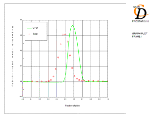
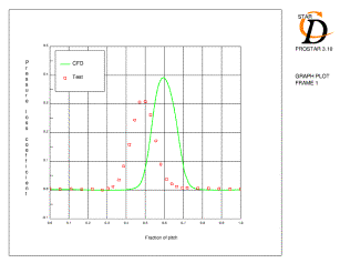
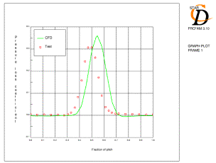
Wake profiles for case 3 at the exit traverse plane for the three meshes are shown in Figure 4.1. The results are plotted from mid-passage to mid-passage (i.e. over the pitchwise extent of the computational domain) from pressure side to suction side. As there is no information confirming the datum position of the experimental results the accuracy of the wake alignment is uncertain. The wake depth is generally over-predicted, although the width is less than experiment at the base of the profile for mesh A. Mesh C gives the best result in terms of wake size and shape.
The results on mesh C for the six operating points are shown in Figure 4.2. Again, wake depth is usually slightly high, but generally agreement with experiment is good. Case 9 (for which under-prediction of overall loss was particularly large) shows a much reduced predicted loss coefficient on the suction side. However, the experimental results do show pitchwise non-periodicity, possibly indicating additional loss from 3D flow features.
Surface pressure distributions
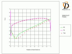
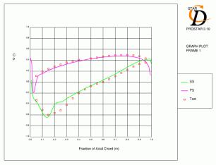
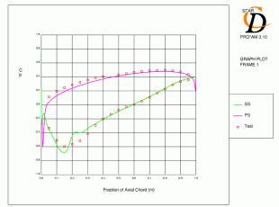
The predictions of surface pressure distribution for case 3 (Figure 4.3) were reasonably accurate for all meshes. The initial deceleration after the suction surface peak was too rapid, which lead to high pressure over the remainder of the blade for meshes A and B. As the minimum pressure on the suction side was slightly low for mesh C, the distribution over the rear of the blade is actually closer. The location of minimum pressure on the suction surface is most accurate for mesh C. At the trailing edge, STAR predicts a small region of negative loading which is due to the acceleration of the pressure side flow around the trailing edge and the separated boundary layer on the suction side. The O-grid topology of mesh C reduces the size of this region to a minimum (see section 4.4).
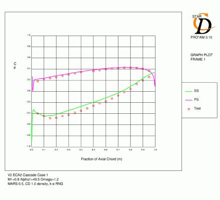
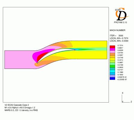
Figures 4.4, 4.5, 4.6, 4.7, 4.8 and 4.9 show contours of Mach number and distribution of pressure coefficient over the blade for all six cases with mesh C. The agreement for the Cp distributions is generally quite good. For cases 1 and 2, which have lower inlet mach numbers, the acceleration over the leading edge region is slightly under-predicted and the subsequent pressure over the rest of the suction surface is high as a result. For the remaining cases with a 0.8 inlet Mach number, the minimum pressure tends to be low and the subsequent diffusion following this peak over-predicted. The location of the suction surface peak and the pressure coefficient at the trailing edge are generally very accurate.
The results for case 9 (Figure 4.8) show similar features to those described above, but the accuracy compared to the experiment is less good. The leading edge loading is increased due to the higher inlet angle (as in case 10) which can be seen in the Mach number contours and the rate of diffusion is significantly higher than the experimental data. The predicted pressure level at the trailing edge is high.
Grid Studies
The boundary layer development from the leading edge is of crucial importance when making accurate predictions of this type of geometry. Improvements over the sheared H grids have been made by changing to an O-type topology to ensure a completely smooth leading edge shape and to improve the orthogonality of the mesh. The recently developed 'ESTurbo' automatic grid generator for turbomachinery geometries provided by the CD-adapco Group has been used to generate such a mesh. But in fact the most significant improvements provided by mesh C appear to be at the trailing edge.
Figure 4.10 and 4.11 show detailed views of flow vectors at the leading and trailing edges for case 3. The trailing edge vectors for mesh A show that the pressure surface flow does not leave the blade at a tangent to the pressure surface, but rather accelerates round the trailing edge circle and hence affects deviation. For mesh C this effect is significantly reduced. The improvements from mesh C are connected with the higher quality cells in this region as well as a better definition of blade shape. In the extreme case of mesh B it can be seen that the trailing edge shape heavily influences the exit flow angle. The effect of different turbulence models on this aspect of the flow could be also be investigated. A higher density O-mesh should also be used to investigate grid independence.
In reality there will be an initial laminar region from the leading edge, with the length of the region and the subsequent transition dependent on the inlet conditions. The use of wall functions in the present model means this boundary layer development cannot be predicted. Improved understanding could be gained by comparison of velocity profiles through the boundary layer with experimental data.
Conclusions and recommendations for future work
The ECA2-V2 linear cascade has been modelled using STAR-CD. The results using simple meshes and standard model settings show that the main flow features are captured and that the overall performance is accurately predicted.
An O-mesh topology around the blade and an H-grid upstream and downstream gives good definition of the blade geometry. In addition, economic clustering of cells in regions of high gradient can be easily achieved. This gave good predictions of deviation and loss at design incidence, although loss was generally slightly low. Deviation in particular improved with the O mesh. Wake profiles were generally slightly deep, with wake width in better agreement. Surface pressure distributions were accurately predicted with locations of suction surface peaks improving with the O mesh.
Boundary layer growth over the blade is a very important aspect of modelling this type of flow. A good definition of the leading edge will help to give the correct flow acceleration and boundary layer thickness as the flow develops. The trailing edge shape can have a strong influence on exit flow angle, especially when unrefined. The O mesh improved this aspect of the model significantly. Higher densities of O-mesh should also be investigated. Improved understanding could be gained by comparison of boundary layer parameters. The use of wall functions with the k-ε turbulence model will become less accurate as the velocity profile differs from the law of the wall, for example during laminar-turbulent transition at the leading edge and in the adverse pressure gradient over the rear of the blade. Further investigations could look at low-Re or two-layer models.
Further work is planned to model the remaining test conditions for which there is experimental data, and to utilise more of the models available within STAR-CD.

© copyright ERCOFTAC 2004
Contributors: Michael Dickens; Alex Read - Computational Dynamics Ltd

