AC 6-10 CFD Simulations
Axial compressor cascade
Application Challenge 6-10 © copyright ERCOFTAC 2004
CFD Simulations
Overview of CFD simulations
The CFD simulations were carried out by Computational Dynamics Limited (CD) as part of an ongoing validation of STAR-CD for turbomachinery applications. The CFD code used was STAR-CD v3.150.
Six test conditions were modelled at which overall performance parameters, blade surface pressure data and wake profiles were compared with experimental data from exit plane traverses. Calculations were performed using two sheared H-meshes and an O-mesh. The number of cells in the blade-to-blade plane ranged from 5500 to 7500. The steady state compressible Navier-Stokes equations using a variant of the k-ε model for closure were solved using the SIMPLE algorithm. Discretisation was undertaken using the second-order MARS scheme with the default compression level of 0.5.
The results show that the main flow features are captured and that the overall performance is reasonably accurate. Deviation and loss were predicted quite accurately for design incidence, although loss was always slightly low. Predicted loss and deviation improved when the O-mesh was used. Surface pressure distributions were in general predicted accurately.
The computational domain covers one blade pitch with the blade located centrally in the domain. The prescribed variation of AVDR enables the case to be modelled using a pseudo-2D approach. This allows the predictions of the fundamental blade-to-blade flow to be evaluated for effects of grid dependency, boundary conditions and numerical settings. The case could also be run fully 3D.
The prediction of boundary layer development in adverse pressure gradients is of central importance to the success of simulations of this type of flow. The experimental data available allows detailed validation of the boundary layer predictions. The STAR-CD code provides a wide range of models and meshing capabilities on which to test this case.
The results are summarised in Table EXP-A and the data contained in these files are given in Table EXP-B.
|
NAME |
|
|
| |||||
|
|
|
|
|
|
|
|
| |
|
CFD 1 |
|
|
|
0.3 |
|
|
|
|
|
|
|
|
|
|
|
|
| |
|
CFD 2 |
|
|
|
|
|
|
|
|
|
|
|
|
|
|
|
|
| |
|
CFD 3 |
|
|
|
|
|
|
|
|
|
|
|
|
|
|
|
|
| |
|
CFD 7 |
|
|
|
|
|
|
|
|
|
|
|
|
|
|
|
|
| |
|
CFD 9 |
|
|
|
|
|
|
|
|
|
|
|
|
|
|
|
|
| |
|
CFD 10 |
|
|
|
|
|
|
|
|
|
|
|
|
|
|
CFD 1 (mesh C) |
|
|
|
|
CFD 2 (mesh C) |
|
|
|
|
CFD 3 (mesh A) |
|
|
|
|
CFD 3 (mesh B) |
|
|
|
|
CFD 3 (mesh C) |
|
|
|
|
CFD 7 (mesh C) |
|
|
|
|
CFD 9 (mesh C) |
|
|
|
|
CFD 10 (mesh C) |
|
|
|
Solution strategy
The CFD simulations were carried out by CD-adapco Group as part of an ongoing validation of STAR-CD for turbomachinery applications. The CFD code used was STAR-CD v3.150. The steady state compressible Navier-Stokes equations using a variant of the k-ε model for closure were solved using the SIMPLE algorithm. Default values for the SIMPLE algorithm relaxation control parameters, residual and solver tolerances were used. The MARS scheme with a blending factor of 0.5 was used to discretise the momentum, total enthalpy and turbulence equations. Full central differencing was used for density interpolation to cell faces. More information is contained in reference 3.1.
Computational Domain
The computational domain, illustrated in Figure 3.1, covers one blade pitch with the blade located centrally in the domain.
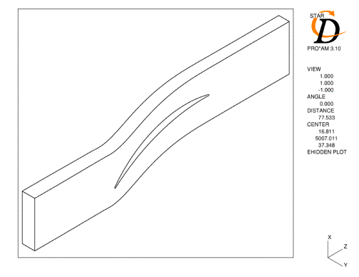
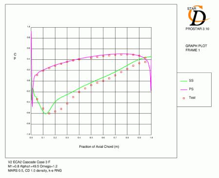
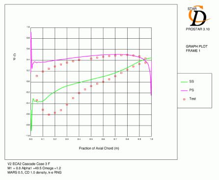
A pseudo-2D approach was adopted and to allow for the endwall effects present in cascade testing, the streamtube thickness was varied by modifying the spanwise position of the endwall boundaries with axial distance. Only an overall value of the streamtube contraction is given in the test data and no information is provided regarding the variation between the inlet and exit planes. To investigate the effect on the predictions, two possible distributions of streamtube thickness were investigated. Firstly an approximately linear variation between the inlet and exit measuring planes and secondly, constant values upstream and downstream and a linear variation between the leading and trailing edges.
Case 3 (M1=0.8, α1=49.5, Ω =1.2) was used to test these distributions. The results (Figure 3.2) show the former approach to be more accurate and this is to be expected for a high aspect ratio (3.75) cascade like the V2. Previous analysis of this cascade confirms these results [3.2].
The variation used is given below:
where: STT=StreamTube Thickness
Ω =Axial Velocity Density Ratio (at exit plane)
x=axial distance
Cax=axial chord
In addition, the effect of the streamtube thickness variation can be analysed by examining the variation in loss with incidence. The mean flow condition at the leading edge will not equal the inlet values due to the streamtube contraction between the inlet measuring plane and the leading edge. A true local incidence value at the leading edge can be evaluated with the above AVDR assumption. Similarly a corrected loss coefficient can be calculated by correcting the measured loss coefficient by the ratio of inlet dynamic heads (p01-p1) at the upstream and leading edge planes. Plotting corrected loss against corrected incidence for the experimental data at 0.8 inlet mach number shows that data points for all operating conditions follow an approximate bucket shaped loss profile (Figure 3.3).
|
Three meshes were used in the study. Mesh A was a sheared-H structure with 7.5k cells and reasonably good leading and trailing edge detail. Mesh B was coarser then mesh A with 6k cells and cusped leading and trailing edges. Mesh C had an O-grid topology around the blade with an H-grid upstream and downstream. This mesh was generated with 4 spanwise cells and had a total of 22k cells with 5.5k in each spanwise layer. Vertices defining the aerofoil section and the extent of the surrounding domain were created using a Fortran program.
The sheared-H meshes were generated manually: splines were fitted through the points and the domain was then filled with 2D cells. The domain extended from x/Cax=-0.53 to x/Cax=1.53, with 150 streamwise points and 50 pitchwise points for mesh A giving a total of 7500 cells. The final mesh was then created by extruding the 2D blade-to-blade mesh in the spanwise direction.
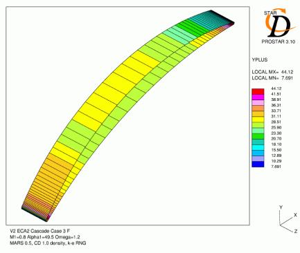
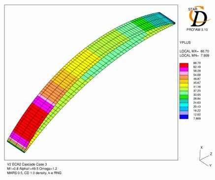
Mesh C was generated using the ESTurbo grid generation package. The O-grid topology around the blade with H-grids at each end gives an excellent blade definition and good cell clustering for an overall low cell count. Therefore it is mainly the results from this mesh that are presented. There were 164 grid points around the blade and 50 across the pitch. The domain was extended to x/Cax=-0.8 to x/Cax=1.8. Mesh points were clustered close to the blade surface and at the leading and trailing edges. Figure 3.4 and Figure 3.5 show detailed views of the meshes at the leading and trailing edges. The mesh was also constructed for best utilisation of wall function boundary conditions, see Figure 3.6.
The wall function representation of the near-wall turbulent behavior is inexact, the accuracy being dependent on the degree to which the assumptions and approximations embodied in the functions correspond with the reality of the application. The main assumptions on which the presently employed wall functions are based are the following:
- Variations in velocity etc. are predominantly normal to the wall, leading to one-dimensional behavior.
- Effects of pressure gradients and body forces are negligibly small, leading to uniform shear stress in the layer.
- Shear stress and velocity vectors are aligned and unidirectional throughout the layer.
- A balance exists between turbulence energy production and dissipation.
- There is a linear variation of turbulence length scale.
More information is contained in Reference 3.1.
Boundary Conditions
The following boundary types and conditions were used:
Stagnation pressure equivalent to 1E5 Pa at the upstream boundary, the inflow angle constrained and a fixed total temperature of 313K. Turbulence intensity was set to 5% and the inlet turbulence length scale to 8E-5.
Fixed static pressure was specified at the outlet such that the appropriate inlet Mach number was achieved.
Cyclic boundaries on the mid-pitch domain boundaries, matched using arbitrary cyclic interfacing.
Adiabatic no-slip walls on the blade surfaces, which were assumed to be hydraulically smooth.
Adiabatic slip-walls (inviscid) on the endwalls.
Application of Physical Models
The flow was assumed to be compressible and steady. Transport equations were solved for two momentum components, total enthalpy, continuity and the turbulence parameters k and ε. The high Reynolds number k-ε RNG turbulence model was used for all the calculations. The fluid properties of air were modelled as follows:
Density: Ideal gas law with molecular weight of 28.96 kg/kmol
Molecular: viscosity Sutherlands Law with μ0=1.71E-5 kg/ms, Cs=116
Specific heat capacity: Constant 1006 J/KgK
Conductivity: Constant 0.026 W/mK
Numerical Accuracy and CPU requirements
The standard convergence criteria (a drop in normalised residuals of three orders of magnitude, and steady monitored values) with standard normalisation was used. Double precision single processor runs were compiled requiring 20MB memory. The runs took on average 1.8 seconds CPU time per iteration on an IBMSP2 and required around 1000 iterations to reach convergence.
Previous experience of similar calculations had shown that meshes 1 and 3 would be an adequate density to capture the flow physics accurately. A coarser mesh of 6000 cells with cusped leading and trailing edges was also run at one test condition for comparison.
Flow Initialisation
Flow initialisation was carried out using the codes built-in initialisation procedure.This procedure endeavors to establish approximate pressure and velocity fields based on a characteristic problem length, supplied specifically for initialisation purposes (the maximum solution domain dimension is taken as the default length). The initial velocities are computed so as to satisfy continuity. In addition, the maximum expected velocity in the solution domain needs to be specified for problems containing only pressure boundaries, or a combination of pressure and total pressure boundaries. The initial velocity field is then scaled to give the specified maximum velocity. In turbulent flow problems, the k and ε fields are initialised using the specified initial distributions of these variables, if available, or the velocity field calculated above, together with turbulence intensity and mixing length specified by the user. For compressible flow, an isentropic density variation assumption is made to compute initial fields of density and temperature from the calculated pressure.
Simulation Case CFD-1
CFD1 V2 cascade simulation: Mesh C. RANS calculations, RNG k-ε, coordinate system as per experiments, cell-centered data. Mass averaging of inlet and exit values for calculations of overall performance. M1=0.3, α1=49.5, Ω=1.2
cfd11.dat (binary file; headers: Re, Tu; L, M1, α1, Ω. columns: Cp)
cfd12.dat (binary file; headers: Re, Tu; L, M1, α1, Ω. columns: ω)
cfd14.dat (binary file; headers: Re, Tu; L, M1, α1, Ω. Data ζ1, M2, a2)
Simulation Case CFD-2
See EXP 1: M1=0.6, α1=49.5, Ω=1.2
Simulation Case CFD-3
See EXP 1: M1=0.8, α1=49.5, Ω=1.2
Also data for mesh A and B.
Simulation Case CFD-7
See EXP 1: M1=0.8, α1=49.5, Ω=1.12
Simulation Case CFD-9
See EXP 1: M1=0.8, α1=52.5, Ω=1.12
Simulation Case CFD-10
See EXP 1: M1=0.8, α1=52.5, Ω=1.3
References
3.1 STAR-CD v3.150 User Guide and Methodology Manuals.
3.2 Application of S1BYL2 to the AGARD WG18 compressor test cases, W.J. Calvert, AGARD CP 510, CFD techniques for propulsion applications, 1991.
© copyright ERCOFTAC 2004
Contributors: Michael Dickens; Alex Read - Computational Dynamics Ltd


