Evaluation AC6-15

Front Page

Description

Test Data

CFD Simulations

Evaluation

Best Practice Advice

Evaluation

COMPARISON OF TEST DATA AND CFD

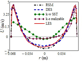
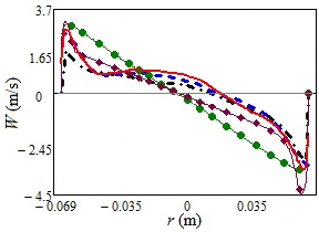
We present first a summary of the performance of various URANS models on a typical RANS grid of 2M nodes and compare with the LES on 6M and DES on 2M grid for the low part-load of ${{\mathcal {Q}}/{\mathcal {Q}}_{n}}$ ≈ 0.4. All RANS calculations were performed in unsteady mode. The time-averaged streamline patterns and colour contours of the fields of the vertical velocity in Fig. 7 clearly show that the RSM, DES and LES all give very similar results; whereas the linear eddy viscosity models (LEVM) show quite a different and, as shown below, erroneous flow pattern. This is substantiated by a quantitative comparison with experiments of the profiles of the axial and tangential velocity components and the rms of their fluctuations at the 3 mm cross-section, Figs 8 and 9. It is noted that the LES on the 6M grid reproduced best the experimental data, but the DES and RSM (both using the coarse, 2M grid) show also good agreement with the measurements. Since the DES employs LES in the flow bulk, it is likely that the LES would also reproduce well the helical vortex pattern on the 2M grid provided the near-wall region (with the average y⁺_1,aver = 9.0) is treated by some wall-function, or using a near-wall RANS approach as practiced by DES. This option was not tested here since, as already stated above, the near-wall resolution on the 2M grid is far too coarse for a proper LES. In contrast, both EVMs notably failed, as shown by typical (unphysical) solid-body profiles of the tangential velocity and a wrong recirculation pattern. Moreover, the k-ε realizable and k-ω SST, LEVMs on the 2M grid could not maintain the unsteadiness, most probably due to excessive numerical diffusion that suppressed the natural instabilities, and resulted in stationary solutions failing to capture the twin rope precessing structures.

k-ε realis. (2M)	RSM (2M)	DES (2M)	LES (6M)
Figure 7: Time-averaged vertical velocity field and streamlines in vertical symmetry plane. The colour denotes the velocity magnitude.

(a)	(b)
Figure 8: Axial (a) and tangential (b) velocity component in the draft tube diffusor at 3 mm behind the cone, obtained by different turbulence models. Grids: (U) RANS and DES 2M, LES 6M.

(a)	(b)
Figure 9: The root-mean-square (rms) of the axial (a) and tangential (b) velocity fluctuations in the draft tube diffusor at 3mm behind the cone obtained by different turbulence models. Grids: (U)RANS and DES 2M, LES 6M. Note: the URANS rms includes both the modelled and resolved contributions, whereas for LES only the resolved rms is shown.

The same prediction quality and trends are observed in the cross section located at 53 mm below the runner (Fig.7, red line) as shown by the velocity profiles and their fluctuations in Figs. 10 and 11. Due to the lack of experimental data at this cross-section we cannot verify the computational data. However, it can be seen that just as in Figs. 8 and 9 for the cross-section of 3 mm, the RSM and DES models are in good agreement with the reference LES results, whereas the results obtained by the two linear EVM models differ significantly showing the same shortcomings as in Figs. 8 and 9.

(a)	(b)
Figure 10: Profile of the axial (a) and tangential (b) velocity component in the draft tube diffusor at 53mm behind the cone obtained by different turbulence models: (U)RANS and DES 2M, LES 6M.

(a)	(b)
Figure 11: The root-mean-square (rms) of the axial (a) and tangential (b) velocity fluctuations in the draft tube at 53 mm behind the cone obtained by different turbulence models. (U)RANS and DES 2M, LES 6M.

However, using a finer grid of 6 M notably improved the performance of the two LEVMs. This time the URANS computations maintained the unsteadiness throughout the whole computations and captured better the characteristic time-averaged streamline pattern and the associated mean velocity profiles, as illustrated in Fig. 12 (here shown for the k-? SST model), comparable to RSM and DES on 2M in Fig. 7. As seen in Fig. 12, the URANS (k-? SST model) computations on 2M grid resulted in a steady solution which differs from those of LES (but also from the k-? realizable model, Fig. 8), whereas the same model on the 6M grid produced unsteady solutions, which after averaging, come much closer to the reference LES pattern.

---

Contributed by: A. Minakov [1,2], D. Platonov [1,2], I. Litvinov [2], S. Shtork [2], K. Hanjalić [3] — 

[1] Institute of Thermophysics SB RAS, Novosibirsk, Russia,

[2] Siberian Federal University, Krasnoyarsk, Russia,

[3] Delft University of Technology, Chem. Eng. Dept., Holland.

Front Page

Description

Test Data

CFD Simulations

Evaluation

Best Practice Advice